Computer Science Dissertations Department of Computer Science
8-9-2016
Real-time In-situ Seismic Tomography in Sensor
Network
Lei Shi
Follow this and additional works at:https://scholarworks.gsu.edu/cs_diss
This Dissertation is brought to you for free and open access by the Department of Computer Science at ScholarWorks @ Georgia State University. It has been accepted for inclusion in Computer Science Dissertations by an authorized administrator of ScholarWorks @ Georgia State University. For more information, please [email protected].
Recommended Citation
by
LEI SHI
Under the Direction of Wenzhan Song, PhD
ABSTRACT
Seismic tomography is a technique for illuminating the physical dynamics of the Earth
by seismic waves generated by earthquakes or explosions. In both industry and academia,
the seismic exploration does not yet have the capability of imaging seismic tomography in
real-time and with high resolution. There are two reasons. First, at present raw seismic
data are typically recorded on sensor nodes locally then are manually collected to central
observatories for post processing, and this process may take months to complete. Second,
impossible due to the sheer data amount and resource limitations. This limits our ability to
understand earthquake zone or volcano dynamics.
To obtain the seismic tomography in real-time and high resolution, a new design of
sensor network system for raw seismic data processing and distributed tomography
compu-tation is demanded. Based on these requirements, three research aspects are addressed in
this work. First, a distributed multi-resolution evolving tomography computation algorithm
is proposed to compute tomography in the network, while avoiding costly data collections
and centralized computations. Second, InsightTomo, an end-to-end sensor network
emula-tion platform, is designed to emulate the entire process from data recording to tomography
image result delivery. Third, a sensor network testbed is presented to verify the related
methods and design in real world. The design of the platform consists of hardware, sensing
and data processing components.
INDEX WORDS: Sensor Network, Seismic Tomography, Distributed Computing,
by
LEI SHI
A Dissertation Submitted in Partial Fulfillment of the Requirements for the Degree of
Doctor of Philosophy
in the College of Arts and Sciences
Georgia State University
by
LEI SHI
Committee Chair: Wenzhan Song
Committee: Xiaojun Cao
Xiaolin Hu
Xiaojing Ye
Electronic Version Approved:
Office of Graduate Studies
College of Arts and Sciences
Georgia State University
DEDICATION
This dissertation is dedicated to Georgia State University. This dissertation is also
dedicated to my parents Tingli Shi and Cuizhen Zhang, for their lasting love, sacrifice and
ACKNOWLEDGEMENTS
This dissertation work would not have been possible without the support of many people.
I want to express my appreciation to my advisor Dr. Wenzhan Song for his kind support and
guidance on my study, research and life. I also want to thank all my committee members,
Dr. Xiaojun Cao, Dr. Xiaolin Hu and Dr. Xiaojing Ye for their kind help and support in
the past several years.
I would like to express my gratitude to Dr. Jonathan M. Lees, Dr. Zhigang Peng and
Dr. Yao Xie for their sincere help and guidance on my research, particularly on some areas
that I have never touched before.
I also want to thank all my friends in the lab for their friendship and help during my
study and research, especially Dr. Mingsen Xu, Dr. Debraj De, Dr. Qingjun Xiao, Dr. Song
Tan, Dr. Liang Zhao and Mr. Goutham Kamath.
Finally I thank NSF for their support with grants 1066391,
TABLE OF CONTENTS
ACKNOWLEDGEMENTS . . . v
LIST OF TABLES . . . viii
LIST OF FIGURES . . . ix
LIST OF ABBREVIATIONS . . . xii
PART 1 INTRODUCTION . . . 1
1.1 First-arrival Traveltime Tomography . . . 2
1.2 Research Background and Focus . . . 3
PART 2 RELATED WORKS . . . 5
PART 3 DISTRIBUTED MULTI-RESOLUTION EVOLVING TO-MOGRAPHY ALGORITHM . . . 11
3.1 Problem Formulation . . . 11
3.2 Algorithm . . . 13
3.2.1 Tomography Partition . . . 14
3.2.2 Multi-resolution Evolving Tomography . . . 17
3.3 Evaluation and Validation . . . 21
3.3.1 Experiment Setup and Implementation . . . 22
3.3.2 Correctness and Accuracy . . . 24
3.3.3 Communication and Computation . . . 27
3.3.4 Data Loss Tolerance and Robustness . . . 29
4.1.1 System Model . . . 30
4.1.2 System Architecture . . . 31
4.2 System Design . . . 32
4.2.1 P-wave arrival time picking . . . 32
4.2.2 Event Location . . . 38
4.2.3 Tomography Inversion . . . 42
4.3 System Implementation. . . 44
4.4 Evaluation . . . 46
4.4.1 P-wave Arrival Time Picking Accuracy . . . 46
4.4.2 Event Location Accuracy . . . 48
4.4.3 Tomography Result . . . 49
PART 5 HARDWARE PROTOTYPE: DESIGN AND OUTDOOR EVALUATIONS . . . 52
5.1 System Design . . . 52
5.1.1 System Architecture . . . 53
5.1.2 Hardware Design . . . 54
5.1.3 Sensing and Data Processing . . . 58
5.1.4 Online Monitoring and Configuration . . . 60
5.2 Data Quality and Picking Accuracy . . . 61
5.2.1 Data Quality . . . 61
5.2.2 P-wave Arrival Time Picking Accuracy . . . 64
5.3 System Evaluation . . . 66
5.3.1 Parkfield 3D Tomography . . . 66
5.3.2 Hammer Shock Field Test . . . 67
PART 6 CONCLUSIONS . . . 72
LIST OF TABLES
LIST OF FIGURES
Figure 1.1 Workflow of 3D First-arrival Traveltime Tomography. . . 2
Figure 1.2 Sensor Network for Seismic Tomography. . . 3
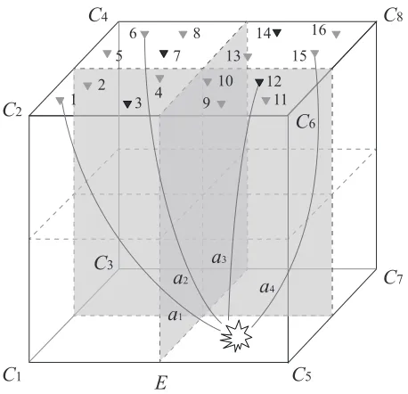
Figure 3.1 Tomography Partition. The resolution of cubeE is 2×2×2 (8 blocks C1 to C8) and 16 sensor nodes are deployed on top of E. . . 14
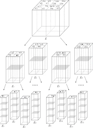
Figure 3.2 Multi-resolution Evolving Tomography. . . 18
Figure 3.3 3D Model in the Simulation. . . 22
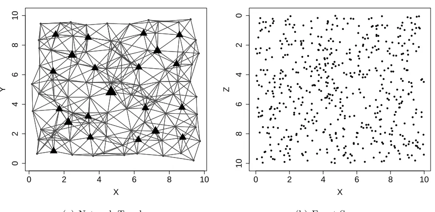
Figure 3.4 Stations and Events Distribution . . . 23
Figure 3.5 2D Tomography Rendering. . . 25
Figure 3.6 Measures of Distance from Synthetic Model. . . 26
Figure 3.7 Communication and Computation Cost Analysis. . . 27
Figure 3.8 Communication and Computation Load Balance. . . 28
Figure 3.9 2D Tomography Rendering with Data Loss. . . 29
Figure 4.1 The Architecture of InsightTomo System. . . 31
Figure 4.2 The seismogram from BHZ channel of four seismometers in Parkfield when an event happens. The vertical lines indicate the manual pickings of P-wave arrival times. . . 33
Figure 4.3 Two Step P-wave Arrival Time Picking. . . 34
Figure 4.5 Spikes that causes change point detection. . . 37
Figure 4.6 Sorted arrival time pickings from 30 stations with the entire day sam-plings on Feb 7, 2002 in Parkfield. . . 40
Figure 4.7 Bundle Layer Architecture. . . 45
Figure 4.8 Performance of Bundle layer vs TCP. . . 46
Figure 4.9 Manual pickings vs algorithm pickings on 6 stations in one event. 47 Figure 4.10 Picking Errors. . . 47
Figure 4.11 1D P-wave Velocity Reference Model. . . 48
Figure 4.12 Event location result comparison, the empty circles and solid disc in-dicate the event location from InsightTomo and the extensive data set respectively. . . 49
Figure 4.13 Horizontal slices of the P-wave velocity at depths of 1, 4, and 7 km. The fault is located around X=13.5km. . . 50
Figure 5.1 Sensor Network System Architecture. . . 54
Figure 5.2 Sensor node in the field. . . 55
Figure 5.3 Hardware components in the box. . . 56
Figure 5.4 Main Hardware Components Connection. . . 57
Figure 5.5 Sensing and Data Processing Framework. . . 58
Figure 5.6 Stream data with arrival time picking on the monitoring and configu-ration tool. . . 60
Figure 5.8 SigmaBox and sensor node deployment. . . 62
Figure 5.9 Waveform of a hammer shock event on sensor node 09 and SigmaBox 69. . . 63
Figure 5.10 Spectrum of the hammer shock event on sensor node 09 and SigmaBox 69. . . 63
Figure 5.11 Signal Noise Level Change . . . 64
Figure 5.12 Audio to Sensor Channel adapter. . . 65
Figure 5.13 Horizontal slices of the P-wave velocity at depths of 2 and 3 km. The fault is located around X=13.5km. . . 66
Figure 5.14 Hammer Shock Test Deployment. . . 68
Figure 5.15 Deployment map of sensor nodes. . . 68
Figure 5.16 Hammer shock event captured. . . 69
Figure 5.17 Hammer shock event captured along the diagonal. . . 70
LIST OF ABBREVIATIONS
• GSU - Georgia State University
• WSN - Wireless Sensor Network
PART 1
INTRODUCTION
Volcanic eruption is one of the most dangerous threats to life on the Earth. In
re-cent years, more volcano activities have drawn the attention of public and scientists. Most
existing volcano monitoring systems employ expensive broadband seismometer as
instru-mentation. Also at present raw seismic data are typically collected at central observatories
for post processing. Seismic sampling rates for volcano monitoring are usually in the range
of 16-24 bit at 50-200 Hz. With such high-fidelity sampling, it is virtually impossible to
collect raw, real-time data from a large-scale dense sensor network, due to severe
limita-tions of energy and bandwidth at current, battery-powered sensor nodes. As a result, at
some most threatening, active volcanoes, fewer than 20 nodes [1] are thus maintained. With
such a small network and post processing mechanism, existing system do not yet have the
capability to recover physical dynamics with sufficient resolution in real-time. This limits
our ability to understand volcano dynamics and physical processes inside volcano conduit
systems. Substantial scientific discoveries on the geology and physics of active volcanism
would be imminent if the seismic tomography inversion could be done in real-time and the
resolution could be increased by an order of magnitude or more. This requires a large-scale
network with automatic in-network processing and computation capability.
To date, the sensor network technology has matured to the point where it is possible to
deploy and maintain a large-scale network for volcano monitoring and utilize the computing
power of each node for signal processing and distributed tomography inversion in real-time.
The methods commonly used today in the procedure of seismic tomography computation
cannot be directly employed under field circumstances proposed here because they rely on
centralized algorithms and require massive amounts of raw seismic data collected on a
mechanism with respect to system design, information processing and tomography inversion
computation.
In this chapter, we first give an introduction on seismic tomography. Then we present
the background and focus of this work and the organization of this dissertation.
1.1 First-arrival Traveltime Tomography
Seismic tomography is a technique for imaging the subsurface of the Earth with seismic
waves produced by earthquakes or explosions. The first-arrival traveltime tomography uses
P-wave first arrival times at sensor nodes to derive the internal velocity structure of the
subsurface. The basic workflow of traveltime tomography illustrated in Figure 1.1 involves
four steps.
Event Location Ray Tracing Tomography Inversion
Sensor Node
Seismic Rays
Estimated Magma Area Blocks on Ray Path Magma
Estimated Event Location Earthquake Event
(b) (c) (d)
P-wave Arrival Time Picking
P-wave
[image:17.612.71.535.339.421.2](a)
Figure 1.1 Workflow of 3D First-arrival Traveltime Tomography.
(a) P-wave Arrival Time Picking. Once an earthquake event happens, the sensor nodes
that detect seismic disturbances record the signals. The P-wave arrival times need to be
extracted from the raw seismic data.
(b) Event Location. The P-wave arrival times and locations of sensor nodes are used to
estimate the event hypocenter and origin time in the volcanic edifice.
(c) Ray Tracing. Following each event, seismic rays propagate to nodes and pass through
anomalous media. These rays are perturbed and thus register anomalous residuals. Given
the source locations of the seismic events and current velocity model, ray tracing is to find
the ray paths from the event hypocenters to the nodes.
(d) Tomography Inversion. The traced ray paths, in turn, are used to image a 3D
into small blocks and the seismic tomography problem can be formulated as a large, sparse
matrix inversion problem.
1.2 Research Background and Focus
This work is part of the project VolcanoSRI (Volcano Seismic Realtime Imaging). This
project aims to create a new paradigm for imaging 4D (four-dimensional) tomography of an
active volcano in real-time. VolcanoSRI is a large-scale sensor network of low-cost geophysical
stations that analyzes seismic signals and computes real-time, full-scale, three-dimensional
fluid dynamics of the volcano conduit system within the active network. The computed 4D
tomography model will illuminate complex, time-varying dynamics of an erupting volcano,
providing a deeper scientific understanding of volcanic processes, as well as a basis for rapid
[image:18.612.76.536.361.561.2]detection of volcanic hazards.
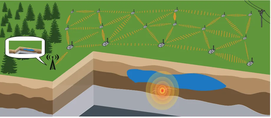
Figure 1.2 Sensor Network for Seismic Tomography.
Realizing the VolcanoSRI system requires a transformative study on the science of
complex volcano systems and the design of large-scale sensor networks. Our approach
in-tegrates innovations on distributed tomographic algorithms, collaborative signal processing
and situation-aware networking technology for large-scale real-time sensor systems. The
performs real-time tomographic inversion within the network. Such an approach has never
been attempted before and represents a major achievement for both earth and computer
science. The team is composed of computer and earth scientists including early pioneers of
wireless sensor networks as applied to volcano monitoring. Figure 1.2 shows the idea for
real-time in-situ 3D tomography computation with VolcanoSRI.
The rest of this dissertation is organized as follows. In chapter 2, we give a survey
of the related works. In chapter 3, we propose the distributed multi-resolution evolving
tomography algorithm for tomography computation. In chapter 4, we present InsightTomo
- an in-situ seismic tomographic imaging system framework in sensor network. In chapter 5,
we give the design and implementation of the testbed system platform. Finally we conclude
PART 2
RELATED WORKS
In this chapter we discuss the related works in the literature of seismic tomography,
solutions for event location, ray tracing, arrival time picking and the least-squares problem.
Static tomography inversion for 3D structure, applied to volcanoes and oil field
explo-rations, has been explored since the late 1970’s [2] [3] [4]. In volcano applications,
tomogra-phy inversion used passive seismic data from networks consisting of tens of nodes, at most.
The development and application to volcanoes include Mount St. Helens [5] [6] [7], Mt.
Rainier [8], Kliuchevskoi, Kamchatka, Russia [9], and Unzen Volcano, Japan [10]. At the
Coso geothermal field, California, researchers have made significant contributions to seismic
imaging by coordinating tomography inversions of velocity [11], anisotropy [12],
attenua-tion [13] and porosity [14].
Sensor network has been deployed for monitoring in many different areas. In [15], the
sensor network was deployed to collect dense environmental and ecological data about
popu-lations of rare species and their habitats. Another sensor system was used by the researchers
to monitor the habitat of the Leach’s Storm Petrel at Great Duck Island [16]. The
Ze-branet [17] project uses sensor network nodes attached to zebras to monitortheir movements
via GPS. It is composed of multiple mobile nodes and a base station with occasional radio
contact. The sensor network was also used to monitor the bridge health [18] [19] and weather
condition as well [20].
For volcano monitoring, The first volcanic monitoring work using WSN was developed
in July 2004 [21], by a group of researchers from the Universities of Harvard, New
Hamp-shire, North Carolina, and the Geophysical Institute of the National Polytechnic School at
Reventador in Ecuador. Data collection was performed with continuous monitoring during
improve the collection of real-time information. The sensor network was deployed on Mount
St. Helens [1] for volcano hazard monitoring and run for months.
P-wave arrival picking has been studied by the community. One widely used approach is
the STA/LTA method [22] that has been using in real deployment [1] on volcano monitoring.
The STA/LTA method continuously monitors the ratio of short-term average over
long-term average on a signal. Since it is based based on RSAM (Realtime Seismic Amplitude
Measurement), which is calculated on raw seismic data samples every second, the accuracy
of STA/LTA method is not enough for tomography computation. Some methods either
determined through joint AR modeling of the noise and the seismic signal [23] or based on
in-network collaborative signal processing [24] are proposed. In seismic tomography, the
event location can also be formulated as a least-squares problem by Geiger’s Method [25].
This problem can be solved by conjugate gradient method or row action method [26]. For ray
tracing, each node can trace the ray paths based on a reference model with either bending
or shooting methods [27] [28] [29] [30] [31]. This can be naturally distributed since the ray
tracing computation is entirely local.
The methods to solve least-squares problem mainly fall into two categories, direct
meth-ods and iterative methmeth-ods. Iterative methmeth-ods for solving large sparse linear systems of
equa-tions are advantageous over the classical direct solvers, especially for huge systems [32].
Methods of parallelizing least-squares solutions on distributed memory architecture have
been studied for both direct and iterative methods, but there are few studies on distributing
the least-squares solutions from a wireless sensor network point of view.
A class of direct solver for least-square problem is through QR decomposition. Strakov´a,
Gansterer and Zemen investigate randomized algorithms based on gossiping for the
dis-tributed computation of the QR factorization [33]. The algorithm is based on modified
Gram-Schmidt orthogonalization (mGS). To distribute the mGS algorithm, they pursue a
randomized decentralized QR factorization algorithm based on gossiping. Gossip-based (or
epidemic) algorithms are characterized by asynchronous randomized information exchange,
the communication is entirely local, the problem is gossiping based algorithm converges slow
and after QR decomposition a back back substitution is required to get the least-square
solution where the nodes need to perform the computation sequentially.
More works have been done on parallelizing iterative algorithms. Renaut proposed a
multisplitting solution of the least-squares problem [34] where the solutions to the local
problems are recombined using weighting matrices to pick out the appropriate components
of each subproblem solution. This algorithm updates the solution by finding the optimal
update with respect to the weights of the recombination. The problem to distribute this
algorithm in the network is that it requires each node to broadcast the residual updates per
iteration. Yang and Brent describe a modified CGLS (MCGLS) method to reduce inner
products global synchronization points, respectively, then improve the parallel performance
accordingly [35]. This can also be potentially distributed over the network but the broadcast
communication is still required per iteration.
In the literature of signal processing, there are a few studies on consensus-based
Dis-tributed Least Mean Square (D-LMS) algorithms [36] [37] [38] [39] [40] [41] in sensor
net-works. These algorithms adopted the weighted sum of local estimations to achieve consensus.
Each sensor node maintains its own local estimation and, to reach the consensus, needs to
continuously exchange the estimation with only its neighbors in the network. Since if the
pro-cess is ergodic and stationary, the least-square estimator approaches the least mean square
estimator as the size of the data set grows, this can also be used for least-square solutions
sta-tistically. The problem is that the consensus-based methods can be slow [42] on convergence
and the communication cost increases along the the estimation vector dimension increases
(in our problem, high resolution seismic has a high-dimension estimation s). Besides, in a
large-scale sensor network, the hop distance between two sensor nodes might be very long.
In such situation, to achieve consensus, any pair of nodes need to exchange high-dimension
estimations frequently. This not only means high communication overhead but also
intro-duces long delays involving many multi-hop communications. Sayed and Lopes developed a
tech-niques that exploit the space-time structure of the data, achieving an exact recursive solution
that is fully distributed [43]. This method requires a cyclic path in the network to perform
the computation on the nodes sequentially and exchanging a dense matrix between nodes.
The most popular iterative method was proposed by Kaczmarz (KACZ) [44] which
is a form of alternating projection method. This method is also known under the name
Algebraic Reconstruction Technique (ART) in computer tomography [45]. This algorithm
do not require the full design of matrix to be in memory at one time and can incorporate new
information (ray paths), on the fly. The vectors of unknowns are updated after processing
each equation of the system and this cycle repeats till it converges. The other variants of
iterative methods are symmetric ART (symART) [46] and Simultaneous ART (SART) [47].
In SymART, one cycle in ART is followed by another cycle in reverse order while in SART,
block of equations are projected instead of just single equation. All these methods are
centralized and cannot be directly applied to distributed seismic tomography.
The block parallel versions of ART have also been proposed and widely used algorithms
among them are component averaging (CAV) [48], Block Iterative- Component Averaging
(BI-CAV) [49] and component-averaged row projections (CARP) [50]. These block-parallel
algorithms use string averaging technique to combine the intermediate result of each block by
taking regular weighted average. The main idea here is to utilize the sparsity of the system
matrix as the weight for averaging. A survey paper comparing various block parallel methods
based on their performance on GPU’s are discussed in [51]. From the above methods, CARP
is more generalized and places no restriction on the system matrix or the selection of blocks.
CARP does not require any pre-processing or pre-ordering of the matrix and provides very
robust method unlike any other block parallel algorithm for solving large sparse linear system.
In CARP, a finite number of KACZ method is applied in each block and the resulting point
in each block is averaged to get next iterate. It is also proved to converge for large scale
systems [50].
In [52] we proposed an algorithm called component average distributed multi-resolution
algorithms such as CAV and CARP for seismic tomography. This was the first algorithm
which was designed to run distributedly to solve tomography problem. Although they were
able to obtain the image it failed to deliver images with sufficient resolution and the
conver-gence stalled after certain iteration. Moreover, their algorithm was developed using regular
grids i.e. the partial differential equation is discretized over a regular cell of same dimensions.
In this paper, our main goal is to show that regular grid partition is not suitable for
dis-tributed tomography and we develop irregular grid method which outperforms CA-DMET in
terms of convergence and also communication overhead. Adaptive mesh refinement (AMR)
has been studied widely and has been used as discretization tool for partial differential
equa-tion as early as 1980 [53]. However, only until early 90’s it was used by seismology community
to solve inverse problem on small set of data [54]. [31] used SVD to interactively change the
boundaries while, [55] used genetic algorithm to optimize the parametrization. These
al-gorithms were suitable for small size data sets and required high computational power to
run efficiently. [56] came up with a less computation intensive solution to parametrize the
coefficient and this algorithm could run efficiently even for large matrices. However, this
algorithm is only suitable for centralized architecture and is not feasible to be implemented
in a distributed scenario.
Here is an analysis of the communication upper bound to distribute some of the methods
mentioned above. For more details about how to distribute the algorithms and the
commu-nication analysis, please refer to our technical report on a survey of distributed least-square
computing in networks [57]. Consider a linear system Ax = b where A ∈ Rm×n(m ≥ n)
and x∈ Rn and b ∈
Rm, a least-squares problem is defined as minx∈Rn||Ax−b||2. The
dis-tributed least-square algorithms can be implemented in a multi-hop networks withN nodes
and converge inO(k) iterations. In D-LMS algorithm,Davg denotes the average node degree
of the network. All the methods above have been proved to be convergent mathematically,
but there are several system design problems for directly applying them in the wireless sensor
networks. In the seismic tomography inversion problem, we intend to solve a large sparse
(hun-Algorithm Communication Cost
1 distributed QR O(kN n2)
2 Multisplitting O(kN2m)
3 distributed MGLS O((k+ 1)N(m+n))
4 D-LMS O(kN(Davg+ 1)n)
5 D-RLS O(N n2)
6 CARP O(2kN n)
Table 2.1 Communication Cost Analysis
dreds of nodes), usually N m and N n. Considering this, the communication cost of
Multisplitting method and CARP is less than other methods if the iteration numbers are in
the same order among these algorithms. But it is hard to bound the iteration numbers of the
methods since it highly depends on the system itself (matrix condition number). Besides,
except for the D-LMS method, other methods either requires broadcast communication per
iteration or a path in the network to perform the computation sequentially on the nodes.
Broadcast communication brings not only high communication cost but also difficulties to
maintain a stable protocol for communication. Since the convergence analysis of these
meth-ods is based on the information completeness, the result is unpredictable if data loss happens
in the communication among iterations. On the other hand, sequential computation along
a path in the network or too many iterations with communication will introduce delays and
may not meet the real-time requirement of the system. In next chapter, we will discuss how
to address these challenges and present an distributed least-square solution which avoids
long-term broadcast communication and delay, at the same time, can still approximate the
PART 3
DISTRIBUTED MULTI-RESOLUTION EVOLVING TOMOGRAPHY
ALGORITHM
In this chapter, we first give the formulation of the seismic tomography computation.
Then we present the distributed multi-resolution evolving tomography algorithm and gives
the formal description of the algorithm. Also, we give an initial evaluation of the proposed
algorithm on correctness, computation and communication cost and tolerance at the end of
this chapter.
3.1 Problem Formulation
Based on the first-arrival traveltime tomography principle discussed in chapter 1. In
To-mography Inversion the volcano is partitioned into small blocks and the seismic toTo-mography
problem can be formulated as a large, sparse matrix inversion problem.
Suppose that there areN nodes andJearthquakes, we consider a perturbation approach
here. Let s∗ be the slowness (reciprocal of velocity) model of the volcano with resolutionM
(blocks). s∗ can be assumed to be a reference model, s0, plus a small perturbation ∆s, i.e.,
s∗ = s0 + ∆s. For simplicity, we use s denote ∆s in the following discussion. The initial
reference model is usually given by the interior layered structure of the earth in seismic
tomography.
We can estimate the ray travel times in Event Location by the arrival times and
esti-mated event origin times. Lett∗i = [t∗i1, t∗i2, . . . , t∗iJ]T, where t∗
ij is the travel time experienced
by nodeiin thej-th event. Based on the ray paths traced in Ray Tracing, the travel time of
a ray is the sum of the slowness in each block times the length of the ray within that block,
i.e., t∗ij =Ai[j, m]·s∗[m] where Ai[j, m] is the length of the ray from the j-th event to node
i in the m-th block and s∗[m] is the slowness of the m-th block. Let t0
be the unperturbed travel times where t0
ij =Ai[j, m]·s0[m]. In the rest of this section, we
use observed travel time and predicted travel time to indicate the same meanings of t∗ij and
t0ij. In matrix notation we have the following equation,
Ais∗−Ais0 =Ais (3.1)
whereAi[j, m] represents the element at thej-th row andm-th column of matrixAi ∈RJ×M.
Let ti = [ti1, ti2, . . . , tiJ]T be the travel time residual such that ti = t∗i −t0i, equation (3.1)
can be rewritten as,
Ais=ti (3.2)
We now have a linear relationship between the travel time residual observations, ti,
and the slowness perturbations, s. Since each ray path intersects with the model only at
a small number of blocks compared with M, the design matrix, Ai, is sparse. The seismic
tomography inversion problem is to solve the system,
As=t (3.3)
where A = [AT
1,AT2, . . . ,ATN]T and t = [tT1,tT2, . . . ,tTN]T. This system is usually
overdeter-mined and the inversion aims to find the least-squares solution s such that,
s= arg min
s kt−As k
2 (3.4)
In seismic tomography, the event location can also be formulated as a least-squares
problem by Geiger’s Method [25], and the estimation vector is of length 4 (event origin time
and 3D coordinates). Since the dimension of the estimation vector is fixed and small, a
centralized solution can be applied in the network for this problem. In Ray Tracing, each
node traces ray path based on a reference model. This can be naturally distributed since the
ray tracing computation is entirely local. The fourth step is the most computationally
can be solved by conjugate gradient method or row action method [26]. However, designed
for high-performance computers, these centralized approaches need significant amount of
computational/memory resources and require the knowledge of global information. As a
result, they cannot be directly distributed in wireless sensor network. Thus, the key research
challenge here is how to solve the least-squares problem in Tomography Inversion
distribut-edly under the severe constraints of wireless sensor network. In this chapter, we focus on
distributed tomography inversion algorithm, while assuming that the event arrival timing
at each node has been extracted from the raw seismic data by each node itself [23] [24], as
well as that the event location and ray tracing have been done. We will discuss more about
arrival timing, event location and ray tracing in chapter 4.
3.2 Algorithm
We developed a new tomography partition and computation distribution algorithm with
a multi-resolution evolving scheme to distribute the computation load, reduce the
communi-cation cost and approximate the least-squares solution of the seismic tomography inversion
problem in the network. To distribute the computation load, we first partition the volcano
structure geometrically and the system As = t correspondingly. Then some nodes are
se-lected as landlords to compute part of the tomography model. The computation on each
landlord is entirely local so that the communication cost is bounded. Since the
computa-tion on each landlord only uses part of the system As = t, the result is not equivalent to
the solution of the original system. To approximate the optimal solution, we introduce the
multi-resolution evolving scheme: the network initially computes a coarse resolution
tomog-raphy without partition when small amount of earthquake events arrive; as more and more
earthquake events arrive, the network will compute finer and finer resolution tomography
with more partitions. The intuition behind this is that the network first computes an outline
of the volcano structure in an low resolution then fills up with finer details inside. With the
multi-resolution evolving scheme, we do not need to wait for all computation done and can
In this section, first we use an example to show the idea of the tomography partition
and the computation distribution over the network; second we introduce the multi-resolution
evolving scheme and give the description of the algorithm.
3.2.1 Tomography Partition
The example in Figure 3.1 illustrates that how to partition the volcano structure
geo-metrically (vertically) and the corresponding systemAs=tfor distributing the computation
in the network.
C1
C6
C2
C3
C5
C7
C8
C4
1 2 3 4 6
7 5
8
910 1211 13
14 15
16
a1
a2
a3
a4
[image:29.612.190.419.260.481.2]E
Figure 3.1 Tomography Partition. The resolution of cube E is 2×2×2 (8 blocks C1 to C8)
and 16 sensor nodes are deployed on top of E.
In this example, cubeE is vertically partitioned into 4 parts (E1 toE4) and there are 4
sensor nodes in each partition, e.g., node 1, 2, 3 and 4 are on top ofE1 consisting of blocksC1
and C2. Suppose that one earthquake happens in blockC5 and node 1, 6, 12 and 15 detect
this event. Once the event location is done, these 4 nodes do ray tracing individually and
get 4 ray paths a1, a2, a3 and a4. Assume that a1 penetrates C5, C1 and C2, a2 penetrates
paths can form a systemAs =t as following,
a1,1 a1,2 0 0 a1,5 0 0 0
a2,1 0 a2,3 a2,4 a2,5 0 0 0
0 0 0 0 a3,5 a3,6 0 0
0 0 0 0 a4,5 0 a4,7 a4,8
·h s1, s2, s3, s4, s5, s6, s7, s8
iT
=h t1, t2, t3, t4 i
T
where al,m is the intersecting length of the l-th ray path and the m-th block, sm is the
slowness perturbation of m-th block, and tl is the travel time residual observation of the
l-th ray path. Notice that each column inA contains the lengths of all the ray paths which
penetrate the corresponding block. So the vertical partition of cube E can be mapped to a
column partition on the systemAs =t,
h
a1,1 a1,2 0 0 a1,5 0 0 0
i
·h s1 s2 s3 s4 s5 s6 s7 s8
iT
=h t1,1 + t1,2 + t1,3 + t1,4
i
where tl,m is the partial travel time residual of the l-th ray path in the m-th block. The
system can be expressed as,
[A1,A2,A3,A4]·[s1,s2,s3,s4]T = [t1+t2 +t3+t4]
whereAp is column partition ofA corresponding to tomography partitionp,tp is the partial
time residuals for Ap, and sp is the partial slowness perturbation model of the blocks in
partition p. Then in each partition, one node is selected as the landlord, e.g., 3, 7, 12 and
and the global tomography can be obtained by combining all sp.
Next is how to partition the travel time residual of each ray. Since the travel time
residual is based on the observation of P-wave arrival time which usually contains noise,
it is difficult to partition the travel time residual exactly for each partial ray. Here an
approximation method is employed to derive the partial travel time residuals based on the
reference model. For example, assume that the reference slowness model forE in Figure 3.1
is s0 = [ˆs
1,ˆs2,sˆ3,sˆ4,sˆ5,sˆ6,ˆs7,sˆ8]T. Let T2 be the observed travel time of ray a2 and the
predicted travel time of a2 is T2(0) = a2 ·s0, thus the travel time residual t2 =T2 −T2(0).
Then the partial predicted travel time can be approximated by the reference slowness model,
T2,1(0) =~a2,1·[ˆs1,sˆ2]T T2,2(0) =~a2,2·[ˆs3,ˆs4]T
T2,3(0) =~a2,3·[ˆs5,sˆ6]T T2,4(0) =~a2,4·[ˆs7,ˆs8]T
where T2,1 is the partial travel time of ray a2 in partition E1,~a2,1 is the part of ray path a2
inE1. The travel time residual then is proportionally partitioned according to the predicted
travel time,
t2,1 =t2·
T2,1(0)
T2(0)
t2,2 =t2·
T2,2(0)
T2(0)
t2,3 =t2·
T2,3(0)
T2(0)
t2,4 =t2·
T2,4(0)
T2(0)
Here we formalize the estimation of the partial travel time residuals. Let ~al,p be the
partial ray path of thel-th ray in partitionEp and lettl,p be the corresponding partial travel
time residual, tl,p can be estimated as,
tl,p=tl·
Tl,p(0)
Tl(0)
the partial slowness reference model of partition Ep then,
Tl,p(0) =~al,p·ˆsp(0)
since tl =Tl−Tl(0) andTl(0) =al·s0, the partial travel time residual tl,p is,
tl,p =Tl·
~al,p·ˆsp(0)
al·s0
−~al,p·ˆsp(0)
The previous discussion explains how to partition the tomography as well as As = t.
Next we will show that how the partition and the computation distribution can be done in the
network. First, after the ray tracing done, each node needs to send the partial ray path and
the estimated partial travel time residual to the corresponding landlords for constructing
the subsystems. Then each landlord can compute the partial slowness perturbation and
broadcast it to the network so that each node can update its reference model part by part
for future ray tracing. So there are two communication patterns in the network, unicast for
sending partial rays and broadcast to synchronize the reference model. Both of them only
happen once in one computation round.
3.2.2 Multi-resolution Evolving Tomography
In this section, we discuss the details about the multi-resolution evolving scheme and
give the description of the proposed algorithm. Figure 3.2 illustrates how the multi-resolution
evolving scheme works following the example in Figure 3.1. Notice that the computation
of the partial travel time residuals highly depends on the slowness reference model. In the
multi-resolution evolving scheme, the tomography model is not partitioned initially so that a
good initial guess of the slowness model can be derived. This initial guess is used to estimate
the partial travel time residuals later for approximating the optimal solution.
Suppose that the resolution of the tomography model isd×d×din the beginning, a single
landlord (node 10 in the example) will compute the first perturbation for the reference model.
4 parts and distributed to 4 landlords (node 3, 7, 12 and 14) for computation as illustrated in
Figure 3.2. Notice that, here the resolution of each partition isd×d×2d. The aforementioned
partition procedure will be recursively applied in each partition when sufficient more new
earthquake events arrive, until the required resolution is achieved. Thus, at the (r+ 1)-th
(r = 0,1,2, . . .) resolution, the tomography model has resolution 2rd ×2rd ×2rd and is
partitioned into 4r parts and evenly distributed to max(N,4r) landlords.
E
E1
1 2 3 4 6
7 5 8
910 1211 1314 1516
1 2 3 4
E2
6 7 5 8
E3
E4
910 1211
1314 1516
1
2
3
4
....
....
9
10
11 12
E1
E2
E3
E4
E9
E10
E11
E12
Algorithm 1Distributed Multi-resolution Evolving Tomography Initialize
1: Node IDid, the resolution level q and dimension d
2: Landlord lists{H1,H2, ...,Hq}
3: r←0, Qr←d×d×d, Pr←1
4: Slowness reference model s0 of resolution Qr
5: Set landlord list to H1, p0 ← the partition index this node locates
6: ifid is equal to hp0
7: rc←0, set the time out threshold Tth
8: endif
Repeat
1: Upon the detection of an event
2: Trace the ray path al, compute~al,p and tl,p for 1≤p≤Pr
3: Send~al,p and tl,p to landlord hp.
4: Upon the reception of~al,p and tl,p
5: if id is equal tohp
6: if rcis equal to 0
7: rc←rc+ 1, start timer Tc
8: else
9: ifTc < Tth
10: Add~al,p and tl,p to Ap0sp0 =tp0
11: else
12: Solve least-squares problem Ap0sp0 =tp0
13: Broadcast sp0 to all other nodes
14: rc←0, resetTc, clear system Ap0sp0 =tp0
15: endif
16: endif
17: else
18: Transfer~al,p and tl,p tohp
19: endif
20: Upon the reception of sp from landlord hp
21: Update the corresponding part of s0 with s
p
22: if allsp(1≤p≤Pr) have been received
23: if r+ 1 is equal to q
24: TERMINATE
25: else
26: r←r+ 1, Q←2rd×2rd×2rd, P ←4r
27: Increase the resolution of s0 toQ
28: Partition the tomography model intoPr parts
29: Set landlord list to Hr+1
30: p0 ←the partition index this node locates
31: ifid is equal to hp0
32: rc←0, set time out threshold Tth
33: endif
34: endif
Now we give the formal description of the Distributed Multi-resolution Evolving
Tomog-raphy (DMET) algorithm, see Algorithm 1. Suppose that there are q different resolution
levels in our multi-resolution scheme, letd be the initial resolution dimension.
At the (r+ 1)-th resolution, the tomography model E with resolution Qr is vertically
and evenly partitioned into Pr different parts, then the p-th part Ep contains Qr/Pr blocks
(Qr = 2rd×2rd×2rd and Pr = 4r). The system As = t can be partitioned by columns
accordingly,
[A1,A2, . . . ,APr]·[s1,s2, . . . ,sPr]T = [t1+t2 +. . .+tPr]
and for Ep the following subsystem is constructed on a landlord,
Apsp =tp
where 1≤p≤Pr.
Initialize line 1-4: Each node initialize its ID, the resolution level qand initial
dimen-sion d. Besides, each node initializes a landlord list {H1,H2, ...,Hq} where Hr+1 is a node
list{hp|1≤p≤Pr}and hp indicates the landlord for partitionpat the (r+ 1)-th resolution.
This tells each node where to send the partial ray information. Then the resolution and
partition parameters and a slowness reference model for ray tracing are initialized.
Initialize line 5-8: Set the landlord list as H1 (only one landlord in it). If this node
is the landlord, it also initializes a ray counter and a time out threshold Tth which controls
the waiting time for a landlord to receive partial ray information from other nodes. Because
it is hard to know how many partial rays will be received by the landlord since the event
activity is unpredictable.
Repeat line 1-3: After the initialization, each node will act based on the event
de-tection and message reception. Once an event is detected by a node, either a landlord or a
common node, it will trace the ray path (as assumed in previous discussion, the event
loca-tion has already been estimated in the network and every node knows it). Then the node
the landlord list Hr+1.
Repeat line 4-19: If the node is a landlord in partition p0, when it receives the
first partial ray for current resolution, the node will start a timer Tc. Otherwise, if the
timer is less than the threshold Tth, the landlord will add the received partial ray into the
subsystemAp0sp0 =tp0. Once the timerTcis out, the node will compute the partial slowness
perturbationsp0 from constructedAp0sp0 =tp0. Then the landlord broadcasts sp0 to all other
nodes and reset the parameters. If the node is not a landlord, it will transfer the received
partial ray information to the corresponding landlord.
Repeat line 20-35: Once a node receives the slowness perturbation sp from landlord
hp. It will update the corresponding part of the slowness reference model s0 with sp. After
the partial slowness perturbations from all landlords have been received, i.e., the entire
slowness reference model has been updated. The algorithm will TERMINATE if the required
resolution is met; otherwise, the node will set r to r+ 1, calculate current Qr and Pr, and
increase the resolution of reference model s0 toQ
r. There are different ways to increase the
resolution of the model, e.g., all the blocks in higher resolution just use the slowness value of
the block it belongs to in the lower resolution. Then each node will partition the model into
Pr parts. Also, the node will set the appropriate landlord list. If the node is a landlord at
(r+ 1)-th resolution, it will initial a ray counter and set a timeout threshold (the threshold
is larger in higher resolution since more rays are needed for higher resolution tomography
computation).
Notice that the algorithm here is based on a cube tomography model, in reality the
model is not always a cube and the partition may depend on the deployment of the sensor
network. This algorithm can be applied to different models, it only needs to change the
resolution evolving and partition scheme, i.e., how to set Qr and Pr in resolution level r.
3.3 Evaluation and Validation
We implemented and evaluated the algorithm with our InsightTomo emulation system,
proposed algorithm not only balances the computation load, but also achieves low
commu-nication cost and good data loss tolerance.
3.3.1 Experiment Setup and Implementation
Our evaluation uses synthetic magma and earthquake events data. First, a data
gen-erator is implemented to generate a magma area and earthquake events. Assume that the
tomography model is a cube of dimension 10×10×10 km. Then we set a predefined magma
area as the ground truth as shown in Figure 3.3. The velocities of seismic waves inside
and outside the magma area are V and 0.9V whereV is 4.5km/s which is a typical P-wave
[image:37.612.208.380.355.521.2]velocity.
Figure 3.3 3D Model in the Simulation.
In InsightTomo emulator, a network of 100 nodes is deployed on the top of the
mon-itoring area. We set the target tomography resolution to be 32×32×32 = 32768 where
each block is of size 0.3215 km3. The data generator then generates earthquake events with
random location and time, and calculates ray travel times from event locations to all sensor
nodes. To simulate the event location estimation and ray tracing errors, a White Gaussian
Each node can calculate the predicted travel time based on the initial model in different
resolutions.
Notice that based on the predefined slowness model for the cubic area, the generator
is supposed to calculate the exact travel time for each ray. But the magma area itself is a
discrete model and the surface shown in Figure 3.3 is constructed from a discrete data set.
So the generator partitions the cube area with a much higher resolution 128×128×128 as
the ground truth and assigns the slowness value to the blocks according whether their center
points are in the magma area or not.
100 stations are randomly distributed on top of the cube and form a mesh network
as shown in Figure 3.4(a) (the black triangles indicate the landlords in different resolution
levels). 650 events are similarly distributed, Figure 3.4(b) which shows the vertical view of
the event sources distribution.
● ● ● ● ● ● ● ● ● ● ● ● ● ● ● ● ● ● ● ● ● ● ● ● ● ● ● ● ● ● ● ● ● ● ● ● ● ● ● ● ● ● ● ● ● ● ● ● ● ● ● ● ● ● ● ● ● ● ● ● ● ● ● ● ● ● ● ● ● ● ● ● ● ● ● ● ● ● ● ● ● ● ● ● ● ● ● ● ● ● ● ● ● ● ● ● ● ● ● ●
0 2 4 6 8 10
0 2 4 6 8 10 X Y
(a) Network Topology
● ● ● ● ● ● ● ● ● ● ● ● ● ● ● ● ● ● ● ● ● ● ● ● ● ● ● ● ● ● ● ● ● ● ● ● ● ● ● ● ● ● ● ● ● ● ● ● ● ● ● ● ● ● ● ● ● ● ● ● ● ● ● ● ● ● ● ● ● ● ● ● ● ● ● ● ● ● ● ● ● ● ● ● ● ● ● ● ● ● ● ● ● ● ● ● ● ● ● ● ● ● ● ● ● ● ● ● ● ● ● ● ● ● ● ● ● ● ● ● ● ● ● ● ● ● ● ● ● ● ● ● ● ● ● ● ● ● ● ● ● ● ● ● ● ● ● ● ● ● ● ● ● ● ● ● ● ● ● ● ● ● ● ● ● ● ● ● ● ● ● ● ● ● ● ● ● ● ● ● ● ● ● ● ● ● ● ● ● ● ● ● ● ● ● ● ● ● ● ● ● ● ● ● ● ● ● ● ● ● ● ● ● ● ● ● ● ● ● ● ● ● ● ● ● ● ● ● ● ● ● ● ● ● ● ● ● ● ● ● ● ● ● ● ● ● ● ● ● ● ● ● ● ● ● ● ● ● ● ● ● ● ● ● ● ● ● ● ● ● ● ● ● ● ● ● ● ● ● ● ● ● ● ● ● ● ● ● ● ● ● ● ● ● ● ● ● ● ● ● ● ● ● ● ● ● ● ● ● ● ● ● ● ● ● ● ● ● ● ● ● ● ● ● ● ● ● ● ● ● ● ● ● ● ● ● ● ● ● ● ● ● ● ● ● ● ● ● ● ● ● ● ● ● ● ● ● ● ● ● ● ● ● ● ● ● ● ● ● ● ● ● ● ● ● ● ● ● ● ● ● ● ● ● ● ● ● ● ● ● ● ● ● ● ● ● ● ● ● ● ● ● ● ● ● ● ● ● ● ● ● ● ● ● ● ● ● ● ● ● ● ● ● ● ● ● ● ● ● ● ● ● ● ● ● ● ● ● ● ● ● ● ● ● ● ● ● ● ● ● ● ● ● ● ● ● ● ● ● ● ● ● ● ● ● ● ● ● ● ● ● ● ● ● ● ● ● ● ● ● ● ● ● ● ● ● ● ● ● ● ● ● ● ● ● ● ● ● ● ● ● ● ● ● ● ● ● ● ● ● ● ● ● ● ● ● ● ● ● ● ● ● ● ● ● ● ● ● ● ● ● ● ● ● ● ● ● ● ● ● ● ● ● ● ● ● ● ● ● ●
0 2 4 6 8 10
10 8 6 4 2 0 X Z
[image:38.612.78.522.377.593.2](b) Event Sources
Figure 3.4 Stations and Events Distribution
We evaluate the algorithm starting with resolution 83 and one partition, evolving to
resolution 163 with 4 partitions and complete at resolution 323 with 16 partitions. 50, 100
overdetermined. To simulate the event location estimation and ray tracing errors, a White
Gaussian Noise is added to the travel time to generate the sensor node observations (arrival
times).
To simulate the sensing behavior of the nodes in the network, two subnetworks are built
in the emulator. One is the wireless mesh network in Figure 3.4(a) with a link and physical
layer connectivity model. The other is a simple wired network where one generator node
wired connects with each node in the mesh network. This generator node will generate event
at random time, compute the travel times from this event to each node based on the ground
truth, and send the event location and travel time to corresponding node with noise (suppose
that the event location has been done as we discussed above). So the nodes in mesh network
are blind to the event activity and thus simulate the sensing behaviour.
The Bayesian version of ART method [58] is used in the experiments to compute the
tomography. We use the relative update of the estimation between two sweeps (one sweep
means that all the ray paths in the system are used once for estimation update) as the
stopping criteria. Besides, a centralized collection scheme (one node collects all the ray
information and perform centralized computation) is implemented in the emulator with
the same data set to compare with our DMET algorithm. Notice that the Bayesian ART
method solves the systemAs=tto minimizekt−Ask2 +λ2 ksk2 whereλis the trade-off
parameter that regulates the relative importance we assign to models that predict the data
versus models that have a characteristic, a priori variance.
3.3.2 Correctness and Accuracy
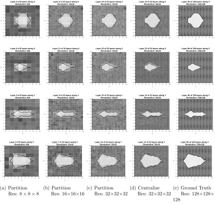
To validate the correctness and accuracy of the algorithm, we first visualize the
tomog-raphy result in vertical slices in Figure 3.5. Each row of figures shows the same tomogtomog-raphy
slice on corresponding layer along with X or Y axes (the total layers of each figure is equal
to the resolution dimension of the result). The black polygons give the cross section outline
of the magma chamber surface. We can see that at the lowest resolution 83, the result can
the small cross section in the first row. But it gives a good start point for the higher
resolu-tion to further refine the result. At resoluresolu-tion dimension 16, the result can closely show the
outline of the magma chamber. The result in column (c) at resolution 323 is already very
close to the centralized solution in column (d).
Y
Z
Layer 3 of 8 layers along X Resolution: 8x8
0 1 2 3 4 5 6 7 8 9 10
10 9 8 7 6 5 4 3 2 1 0 Y Z
Layer 5 of 16 layers along X Resolution: 16x16
0 1 2 3 4 5 6 7 8 9 10
10 9 8 7 6 5 4 3 2 1 0 Y Z
Layer 10 of 32 layers along X Resolution: 32x32
0 1 2 3 4 5 6 7 8 9 10
10 9 8 7 6 5 4 3 2 1 0 Y Z
Layer 10 of 32 layers along X Resolution: 32x32
0 1 2 3 4 5 6 7 8 9 10
10 9 8 7 6 5 4 3 2 1 0 Y Z
Layer 40 of 128 layers along X Resolution: 128x128
0 1 2 3 4 5 6 7 8 9 10
10 9 8 7 6 5 4 3 2 1 0 Y Z
Layer 6 of 8 layers along X Resolution: 8x8
0 1 2 3 4 5 6 7 8 9 10
10 9 8 7 6 5 4 3 2 1 0 Y Z
Layer 11 of 16 layers along X Resolution: 16x16
0 1 2 3 4 5 6 7 8 9 10
10 9 8 7 6 5 4 3 2 1 0 Y Z
Layer 22 of 32 layers along X Resolution: 32x32
0 1 2 3 4 5 6 7 8 9 10
10 9 8 7 6 5 4 3 2 1 0 Y Z
Layer 22 of 32 layers along X Resolution: 32x32
0 1 2 3 4 5 6 7 8 9 10
10 9 8 7 6 5 4 3 2 1 0 Y Z
Layer 88 of 128 layers along X Resolution: 128x128
0 1 2 3 4 5 6 7 8 9 10
10 9 8 7 6 5 4 3 2 1 0 X Z
Layer 3 of 8 layers along Y Resolution: 8x8
0 1 2 3 4 5 6 7 8 9 10
10 9 8 7 6 5 4 3 2 1 0 X Z
Layer 5 of 16 layers along Y Resolution: 16x16
0 1 2 3 4 5 6 7 8 9 10
10 9 8 7 6 5 4 3 2 1 0 X Z
Layer 10 of 32 layers along Y Resolution: 32x32
0 1 2 3 4 5 6 7 8 9 10
10 9 8 7 6 5 4 3 2 1 0 X Z
Layer 10 of 32 layers along Y Resolution: 32x32
0 1 2 3 4 5 6 7 8 9 10
10 9 8 7 6 5 4 3 2 1 0 X Z
Layer 40 of 128 layers along Y Resolution: 128x128
0 1 2 3 4 5 6 7 8 9 10
10 9 8 7 6 5 4 3 2 1 0 X Z
Layer 4 of 8 layers along Y Resolution: 8x8
0 1 2 3 4 5 6 7 8 9 10
10 9 8 7 6 5 4 3 2 1 0 (a) Partition Res: 8×8×8
X
Z
Layer 7 of 16 layers along Y Resolution: 16x16
0 1 2 3 4 5 6 7 8 9 10
10 9 8 7 6 5 4 3 2 1 0 (b) Partition Res: 16×16×16 X Z
Layer 14 of 32 layers along Y Resolution: 32x32
0 1 2 3 4 5 6 7 8 9 10
10 9 8 7 6 5 4 3 2 1 0 (c) Partition Res: 32×32×32 X Z
Layer 14 of 32 layers along Y Resolution: 32x32
0 1 2 3 4 5 6 7 8 9 10
10 9 8 7 6 5 4 3 2 1 0 (d) Centralize Res: 32×32×32 X Z
Layer 56 of 128 layers along Y Resolution: 128x128
0 1 2 3 4 5 6 7 8 9 10
10 9 8 7 6 5 4 3 2 1 0
[image:40.612.86.524.180.597.2](e) Ground Truth Res: 128×128× 128
Figure 3.5 2D Tomography Rendering.
Using ˜s, s∗ and ¯s to represent the synthetic model, the reconstructed model and the
0 0.2 0.4 0.6 0.8 1
DMET(8) DMET(16) DMET(32) CENT(32)
Error
Scenarios
e1
(a)
0 0.02 0.04 0.06 0.08 0.1
DMET(8) DMET(16) DMET(32) CENT(32)
Error
Scenarios
e2 e3
(b)
Figure 3.6 Measures of Distance from Synthetic Model.
the synthetic model provided in [26] to evaluate the estimation quality,
e1 = (
Xn
i=1(˜si−s
∗
i)
2 /
n X
i=1
(s∗i −¯s)2)12
e2 =
Xn
i=1|˜si−s
∗
i|/
Xn
i=1|s
∗|
e3 = max|˜si−s∗i|
These represent the normalized root mean squared distance, the average absolute value
distance and the worst case distance respectively. The result is shown in Figure 3.6,
DMET(8) means that the distance analysis of DMET algorithm with resolution 83 and
CENT(32) indicates the result of centralized algorithm. First we observe that in DMET
al-gorithm, the distances are decreasing along with the increase of the resolution. The distances
in DMET(32) are even smaller than CENT(32), this is because that we use the relative
up-date as the stop criteria in Bayesian ART method and the centralized algorithm may stop
before the distance is small enough. This analysis can imply that the multi-resolution
evolv-ing scheme can give a good approximation on each resolution level for estimatevolv-ing partial
travel times and the computation can approximate the centralized solution while not
3.3.3 Communication and Computation
From the experiment result and analysis, it is validated that DMET gives a good result
to approximate the tomography compared with the centralized algorithm. Next, we will
compare the communication and computation cost between DMET and the centralized
al-gorithms. Since the ray tracing algorithm is very expensive to perform, we assume that each
node does ray tracing itself and sends the indexed ray path to a base station (centralized)
or to the corresponding landlords. Also, after centralized computation done on the base
station, it will broadcast the model to the network for future ray tracing since the whole
tomography process is iterative.
0 2e+08 4e+08 6e+08 8e+08 1e+09 1.2e+09
DMET(8) DMET(16)DMET(32) DMET(T) CENT(M) CENT(C)
Communication Volume (bytes)
Scenarios
Unicast Broadcast Total
(a) Communication
0 1e+09 2e+09 3e+09 4e+09 5e+09 6e+09
DMET(8) DMET(16) DMET(32) DMET(T) CENT(M) CENT(C)
Arithmetic Operations
Scenarios
(b) Computation
Figure 3.7 Communication and Computation Cost Analysis.
Figure 3.7 gives the communication and computation cost analysis where DMET(T) is
the total cost for DMET algorithm, CENT(M) and CENT(C) are the cost of centralized
algorithm when the base station is in the center and the corner of the network respectively.
In Figure 3.7(a), we can see that the total unicast cost of DMET is much less than centralized
algorithm (about one third of CENT(C)) since the centralized data collection will cause more
interference and congestion when the data rate is high. At the same time, the broadcast cost
of DMET is more than centralized algorithm because multiple nodes need to broadcast in
landlords, Figure 3.7(c) gives the computation cost for centralized algorithm and DMET.
The total cost of DMET is higher than centralized since we partition and distribute the
system to landlords, and the computation on landlords are entirely local and it is lack of the
global information to constraint the problem for fast convergence.
0 1 2 3 4 5 6 x 10⁷
0 2 4 6 8 10 0 5 10 0 1 2 3 4 5
x 107
C o mmu ni c a ti o n V o lu me
(a) CENT(M) Communication
0 1 2 3 4 5 6
x 107
0 2 4 6 8 10 0 5 10 0 1 2 3 4 5 6
x 107
C o mmu ni c a ti o n V o lu me
(b) CENT(C) Communication
0 2 4 6 8 10 0 5 10 0 2 4 6x 10
7 Communication Volum e 0 1 2 3 4 5 6 x 10⁷
(c) DMET Communication
0 5e+08 1e+09 1.5e+09 2e+09 2.5e+09 3e+09
1 12 16 23 24 28 33 37 45 49 52 56 64 68 73 77 78 85 89
Arithmetic Operations
Node ID
[image:43.612.89.519.176.483.2](d) Computation
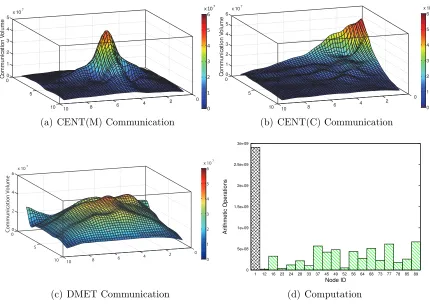
Figure 3.8 Communication and Computation Load Balance.
The experiment results above have shown that the total communication cost of DMET
is less than the centralized algorithm while the total computation cost is higher. Next, we
count the communication and computation cost on each node in the network to show that
DMET balances the communication and distribute the computation load in the network.
Figure 3.8(a), (b) and (c) visualize the communication cost on each node in the network
for 3 different scenarios with heat maps. From Figure 3.8(a) and (b), we can see that the
communication cost in centralized scenario for the nodes near the base station (either in the
through them. The communication cost on each node in our algorithm shown in Figure 3.8(c)
is more balanced. In Figure 3.8(d), the first column is the computation load on node 1 for
CENT(C) algorithm, all other columns are the computation load on corresponding landlords
of DMET algorithm. We can see that although the total computation cost of DMET is higher
but the computation load is much more balanced.
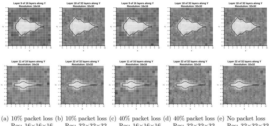
3.3.4 Data Loss Tolerance and Robustness
We did an evaluation on the robustness of DMET. The algorithm runs with the same
data set and two different packet loss ratios of 10% and 40% set in the emulator. Figure 3.9
gives part of the 2D slice rendering along Y axes with packet loss. From Figure 3.9, we can
see that with 10% or even 40% packet loss, compared to the result without packet loss there
is not much difference in terms of the magma area outline. This validate the robustness of
DMET algorithm which can be tolerant to a severe packet loss.
X
Z
Layer 9 of 16 layers along Y Resolution: 16x16
0 1 2 3 4 5 6 7 8 9 10
10 9 8 7 6 5 4 3 2 1 0 X Z
Layer 18 of 32 layers along Y Resolution: 32x32
0 1 2 3 4 5 6 7 8 9 10
10 9 8 7 6 5 4 3 2 1 0 X Z
Layer 9 of 16 layers along Y Resolution: 16x16
0 1 2 3 4 5 6 7 8 9 10
10 9 8 7 6 5 4 3 2 1 0 X Z
Layer 18 of 32 layers along Y Resolution: 32x32
0 1 2 3 4 5 6 7 8 9 10
10 9 8 7 6 5 4 3 2 1 0 X Z
Layer 18 of 32 layers along Y Resolution: 32x32
0 1 2 3 4 5 6 7 8 9 10
10 9 8 7 6 5 4 3 2 1 0 X Z
Layer 11 of 16 layers along Y Resolution: 16x16
0 1 2 3 4 5 6 7 8 9 10
10 9 8 7 6 5 4 3 2 1 0
(a) 10% packet loss Res: 16×16×16
X
Z
Layer 22 of 32 layers along Y Resolution: 32x32
0 1 2 3 4 5 6 7 8 9 10
10 9 8 7 6 5 4 3 2 1 0
(b) 10% packet loss Res: 32×32×32
X
Z
Layer 11 of 16 layers along Y Resolution: 16x16
0 1 2 3 4 5 6 7 8 9 10
10 9 8 7 6 5 4 3 2 1 0
(c) 40% packet loss Res: 16×16×16
X
Z
Layer 22 of 32 layers along Y Resolution: 32x32
0 1 2 3 4 5 6 7 8 9 10
10 9 8 7 6 5 4 3 2 1 0
(d) 40% packet loss Res: 32×32×32
X
Z
Layer 22 of 32 layers along Y Resolution: 32x32
0 1 2 3 4 5 6 7 8 9 10
10 9 8 7 6 5 4 3 2 1 0
[image:44.612.84.523.383.589.2](e) No packet loss Res: 32×32×32
PART 4
END-TO-END SYSTEM DESIGN AND EMULATION
In traditional seismology, the raw seismic data is collected for manual analysis including
P-wave arrival time picking on the seismograms. Then centralized methods will process the
data and compute seismic tomography. Keep in mind that our goal is to design a system
which can deliver 3D tomography in real-time over a large-scale sensor network by utilizing
the limited communication ability in the network and the computation power on the sensor
node. To reach this goal, first no raw seismic data should be transmitted over the network,
which requires a light weighted algorithm that can accurately pick the P-wave arrival time
on the sensor nodes locally inside the network. Second, an efficient distributed tomography
computation method is needed for processing data and inverting volcano tomography in the
network while avoiding both costly data collections and centralized computations.
In this chapter we present InsightTomo - an in-situ seismic tomographic imaging system
framework in sensor network. The design of InsightTomo consists of a series of algorithms
and network design to automatically process the seismic data, pick the P-wave arrival time,
identify seismic events and compute the seismic tomography in-situ in real-time. The system
design is evaluated with real data from the San Andreas Fault (SAF) on Parkfield.
4.1 System Overview
4.1.1 System Model
The mesh network architecture is employed in the design of InsightTomo. Each sensor
node in the network is equipped with a seismic sensor (e.g., single or three component
geophone) that continuously samples and records the signal in an external storage (e.g., SD
memory card). Also, the sensor node has a low power MCU (e.g., MSP-430 or Imote series)
the sensor nodes have GPS modules on board [1] such that the clocks on sensor nodes are
time-synchronized so are the time pickings. A powerful computation unit (e.g., BeagleBone
Black board, cellphone or tablet) is also installed on each node; the unit can complete the
computation-intensive tasks including the event location and tomography inversion.
4.1.2 System Architecture
In this section, we will give an overview of the system architecture and the data flow
of InsightTomo respect to the design requirements mentioned above. InsightTomo consists
of several algorithms running on sensor nodes and coordinator nodes, and a bundle layer
protocol is proposed to improve the performance of communication. Figure 4.1 illustrates the
architecture and dataflow of InsightTomo system. There are three steps in the architecture
corresponding to the workflow of seismic tomography.
Sensor 1
P-wave arrival time picking
Sensor 2
P-wave arrival time picking
Sensor J
P-wave arrival time picking
. . .
Coordinator
Event
Identi
c
ation
E
v
en
t
L
o
ca
tio
n
Sensor 1
Ray Tracing
Sensor 2
Ray Tracing
Sensor J
Ray Tracing
. . .
Landlord
Tomography Inversion
Landlord P
Tomography Inversion
. . .
Sensor 1
Combine & Update Model
Sensor 2
Sensor J
. . .
Combine & Update
Model
Combine & Update Model
Figure 4.1 The Architecture of InsightTomo System.
(1) Sensor node receives the signal from the sensor and analyze the signal with P-wave
arrival time picking algorithm. The algorithm will continuously monitor the samplings and
alarm if an event is detected, then the picking algorithm will pick the P-wave arrival time.
After the arrival time picking done, the sensor node only needs to send the arrival time to