The research of the knee joint’s motion model based on the kinetic equation of multi body system

(1)

Journal of Chemical and Pharmaceutical Research, 2013, 5(11):164-171

Research Article

_{CODEN(USA) : JCPRC5}

ISSN : 0975-7384

The research of the knee joint’s motion model based on the kinetic equation of

multi-body system

Shan Fan and Mei Wang

Zhejiang Industry & Trade Vocational College, Wenzhou, Zhejiang, China

_____________________________________________________________________________________________

ABSTRACT

During physical exercise, the knee is vulnerable to injuries. In order to prevent such injuries, many people have analyzed knee pads and sports biomechanics of knee. This paper studies the simulation model of knee joint motion. On the basis of analysis on the geometric model of the knee joint during exercise, it establishes the dynamic equations of knee joint motion and obtains the mechanics response function of knee joint muscle, discusses the change trends of the angle and the angular velocity over time by biomechanical simulation data of knee joints and related systems in the starting process, verifies the reliability of the model through the simulation results, and provides a theoretical basis for medicine and sports to prevent damage.

Key words: Human physiology, Kinetic equation, Response function

_____________________________________________________________________________________________

INTRODUCTION

Organizations around the knee are more complex, and the functions between these structures are mutually interacted. During physical exercise the knee is susceptible to injury, and this injury is often not easy to recover, so excellent potential athletes have to retire. The current research for knee injury mostly stays in level of experience prevention and injury treatment [1, 2]. If we can accurately determine the biomechanical parameters of the knee joint and each structure during movement and the material mechanical parameters of substance itself, which may have better results to prevent knee injury [3, 4]. For exploring the movement of the knee joint, this paper thinks that the use of computer simulation can receive better benefits. In the calculation simulation process of body structure it requires not only the accuracy of simulation software and hardware reliability, but also need to select the appropriate dynamic model. This paper studies the simulation model for knee motion [5, 6].

Model research is generally divided into physical and mathematical modeling process. The physical model is based on experience and theoretical derivation results, which is easy to understand in the operation and realization and has the advantages of high accuracy; while mathematical modeling is the nature mean of the physical model derivation [7, 8]. When the physical model can not meet the need for simulation, you should use the most essential mathematical methods for its modeling; the ultimate goal and method of theoretical description in mathematical modeling is essentially taking the complex problems as simple questions, and then resolve the problem using mathematical method [9].

(2)

1.The dynamics model principle of computer multi-body system

The dynamics modeling method of computer multi-body system is mainly divided into physical models and mathematical models, wherein physical models refer to build a physical model by the geometry model, and then increase the technical constraints of the kinematics for the geometric model, finally form the physical model that expresses mechanical properties; meanwhile the building form and solving process of the model is also an important symbol of mathematical modeling.

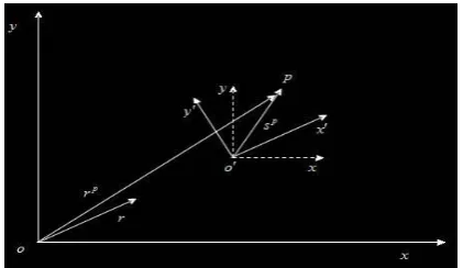
[image:2.595.201.412.197.319.2]

When determining the movement of any point in the multi-body system, you need to transform a point on the study object from the body-fixed coordinate system to the global coordinate system; the coordinate transformation in two-dimensional space is illustrated in Figure 1:

Figure 1: The coordinate transformation chart in two-dimensional space

If the expression of the vectors



in thexoy coordinates and the xoycoordinate system is shown in the formula (1), then point p in Figure 1 has the transformation relation in the formula (2).









   

 



 

T y x

s s s

, ,

 

(1)

p p

p

s r s r

r      A (2) In Formula (2) rp_{represents the coordinates of point} p _{in the global coordinate system,} r_{means the coordinates}

of the origino of the body-fixed coordinate system in the global coordinate system,

p

s _{means the coordinates of}

the vectors



in the global coordinate system,

p

s _{means the coordinates of vector} s_{in the body-fixed coordinate}

system, A _{means the rotational transformation matrix, wherein the form of the rotational transformation matrix is}

in the formula (3).

 

_

  



 

 

 



cos sin

sin cos

A

A (3)

If the time derivative of the matrixA _{is as the formula (4), the global coordinates of any point in the body-fixed}

coordinate system can be obtained, and the transformation formula is in the formula (5).

B

A 

 

  

 _

   

 

  

 

sin cos

cos sin

A d

d

(4)

p p

p

s r s r

r   A   B  ₍₅₎

Then solve the time derivative of the formula (5), acceleration conversion formula at any point can be derived, as shown in the formula (6).

p p

p

s s

r s s

r

r  B  B   B  2A 

(3)

affects the coordination between muscles of the knee joint movement. The following respectively expounds the geometric model, static and quasi-static model and kinetic equations of the knee joint.

3.1 The geometry model of knee joint

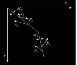
Knee joint has four ligaments. This organizational structure restricts the tibial forward and rearward displacement of the knee joint, which can only rotate in the sagittal plane. The muscles that impact knee joint motion are quadriceps muscles, biceps femora’s, and gastronomies muscle. These muscles are the muscles striding the knee joint, has a direct relationship with the knee joint. Meanwhile quadriceps muscles and biceps femora’s also cross the hip joint; if the knee joint is simplified as viscoelastic hinge, hinge exist the torque generated by the soft tissue effects. Meanwhile the muscles is simplified to facilitate, through the anatomical knowledge on muscle and the corresponding skeletal, the muscle force direction of muscle maintain a slight change with the skeleton, and this change has little to do with the corresponding angle. So: the muscle forces at the connection point of the two muscles and bone is represented by the unidirectional force, the direction of these forces changes with the spatial orientation of the bone, and the relative direction to connecting skeletal muscle stays unchanged. The simplified force diagram of knee joint is shown in Figure 2.

Figure 2: The force analysis diagram of knee joint

[image:3.595.242.373.256.366.2]

The five forces in Figure 2 are the simplified force for human lower limb muscle, and the lower limbs links are divided as shown in Table 1.

Table 1: Lower limb link

Link Demarcation point between links Measuring point from the centroid Proximal point Distal point

Thigh Bone spines point Tibial point Tibial point

Calf Tibial point malleolus medialis point malleolus medialis point

The model parameter of lower limbs is shown in Table 2.

Table 2: The model parameters of human lower limb

Item Symbolic representation Unit Value

Thigh-length l1 m 0.48

Calf and foot length l2 m 0.362

Thigh mass m1 kg 7.727

Calf and foot mass

2

m kg 3.149

Rotational inertia of thigh

1

J kg·m2 0.11794

Rotational inertia of calf and foot J₂ kg·m2 0.0198

Centroid position of the thigh l_m₁ m 0.247

Centroid position of calf and foot l_m₂ m 0.19

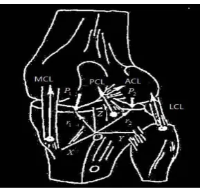
3.2 Knee joint static and quasi-static model

(4)

[image:4.595.234.379.69.211.2]

Figure 3: Hefzy and Grood knee joint model

The ACL, PCL, MCL and LCL in Figure 3 respectively denote anterior cruciate ligament, posterior cruciate ligament, median cruciate ligament and lateral cruciate ligaments. The tensions corresponding to the four ligaments

are respectivelyF1,F2,F3,F4_{. The contact force by the intermeshing of femur and tibia is}P1,P2_{. Through the}

contact force of the four knee joint’s ligament tension and engaging to maintain the balance of the knee joint. As

shown in Figure 3, the spatial coordinate systemO XYZ is established on the tibia, the equilibrium equations are in formula (7) below.

    

     

  



0 0

2 2 1 1

2 1

n

n n T n

n

P r P r F r

P P F

(7)

3.3 The kinetic equation of knee joint

This paper uses the model phenomenon, fixes the pelvis, releases femur and tibia; the hip and knee joint use viscoelastic hinges; add force couple on the hinge to describe the soft tissue effect of the joint, add obstruct force couple to the knee joint to describe the effect that the knee joint cannot bend forward due to the existence of the patella and the structure of ligaments at the knee joint, the foot and tibia are fixedly connected, it can be seen as a rigid body, which has similarities with Lindbeck model and both of them use double pendulum structure, the structure is shown in Figure 4:

Figure 4: The simplified diagram of the knee joint model

In Figure 4 take the hip joint as the coordinate origin, take the front and upward of people as the axis to establish

global coordinate system. The movement of the moving system



x,y



relative to the fixed coordinate system can

be represented by the angle1_{between the femur centerline and the}y _{axis. The movement of the moving}

system



x,y



relative to the moving system



x,y



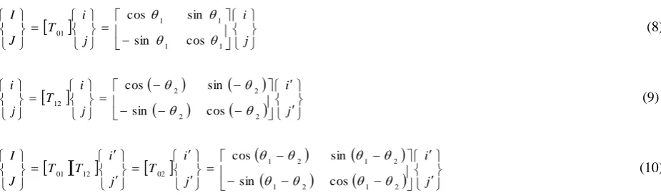
can be represented by the angle 2_{between the center line of}

[image:4.595.205.409.477.623.2]

(5)

 

                           j i j i T J I 1 1 1 1 01 cos sin sin cos     (8)

 

















_                                j i j i T j i 2 2 2 2 12 cos sin sin cos     (9)

  

 

















_                                           j i j i T j i T T J I 2 1 2 1 2 1 2 1 02 12 01 cos sin sin cos         (10)

In the above three formulas the subscript 0,1,2 respectively represent pelvis, femur and tibia, thus the dynamic governing equation of the lower limbs is shown in formula (11), (12), (13) and (14):

 

N m x

F _x

j

x j

j 2

5 4  





 (11)

 

N m y

F _y

j

y j

j 2

5 4  





 (12)

 

   

5

 

  



₂



₁ ₂



4 02 02

1     

    _        

_

 J F T N T M j j j j

B (13)

 

   

3

 

  



₁ ₁

 

₁ ₁ ₁

1 01 01

0    sin  

  J M g m l F T N T M _p j j j j

B       









(14)

In the above four formulas(11) - (14), j

means the unit vector along the longitudinal direction of the jth

muscle;;J1_{means the rotational inertia of the mass center of the femur relative to the hip joint;} J2_{means the}

rotational inertia of the calf and bone’s mass central of foot; Fj

represents the jth muscle tension of the knee

joint; B_{means the position vector of the knee hinge point}B _{in the}



x, y



_{coordinate system;}  j_{denotes the}

position vector of jth muscle’s attachment point in the



x,y



coordinate system; j

denotes the position vector

of jth muscle’s attachment point in the



x, y



coordinate system; B _{means the position vector of the knee}

hinge pointB _{in the}



x, y



_{coordinate system;} l1_{means the length from the mass center of femur to the hip}

joint; M 0_{means the soft tissue effects at the structure of hip joint;}M1_{means the moment caused by the soft}

tissue effect of human knee joint.

4. Data empirical analysis 4.1 Parameter Value situation

[image:5.595.74.537.72.209.2]

All parameter values of the governing equations are as shown in Table 3.

Table 3: All parameter values of the governing equations

Parameter Parameter Value Parameter Parameter Value

1





2 , 2



2

 _0 .0 6 2 , 0 .1 3_m

2

  2 , 2

3

 _0 .0 8 1, 0 .1 4 2_m

3

 0 , 1  ₄ 0 .0 6 , 0 .0 3 3m

4

 0 ,1

5

  0 .0 6 1, 0 .1 2m

5

 0 , 1 _B 0 ,0 .2 4 7m

1

 0 , 0 .1 5m

B

(6)

4.2 The motion simulation data of knee joint

This research studies the knee movement situation during the starting process; the initial position of the study object is the fighting force posture, in which one leg is fixed on the ground, the other leg lifts taking the pelvis as fixed point. People’s hip joint always makes actions of body bent at hips, and the knee joint first bends and then stretches. During the movement simulation, the muscles of the model are activated in stages, and the output function of the muscle force is as formula (15) below.

  m ax 2 1 2 0

1 t kF f , F f

F     (15)

In Formula (15) f1

 

t _{means the function of the muscle’s activation time,} f2



1,2



_{means the force expression}

functions of different muscles, and the values of the two functions during the simulation process are as formula (16) and (17) below.

                 4 . 0 2 . 0 1 , 1 , 1 , 0 , 1 2 . 0 0 0 , 0 , 0 , 0 , 1 15 14 13 12 11 15 14 13 12 11 t f f f f f t f f f f f (16)                                                                  2 exp 2 exp 2 exp 2 exp 2 exp sin 2 exp sin 2 1 24 2 1 23 24 2 23 1 22 1 1 21               f f f f f f (17)

[image:6.595.73.292.227.369.2]

The remaining parameters corresponding to five muscles are shown in Table 4.

Table 4: The remaining parameters corresponding to five groups of muscles

The first group of muscles

The second group of muscles

The third group of muscles

The fourth group of muscles

The fifth group of muscles

k 0.5 0.5 0.1 0.1 0.2

m a x

F ₄₆₈₀ ₁₀₅₀ ₄₅₀₀ ₁₅₀₀ ₅₀₀

0

F 200 100 20 20 20

The data of hip joint angle changing with time is shown in Table 5.

Table 5: The data of hip joint angle changing with time

Time(s) 0.0 0.05 0.10 0.15 0.20 0.25 0.30 0.35 0.40

Angle(rad) 0.00 0.02 0.06 0.14 0.24 0.35 0.50 0.70 0.91

The change trend of the hip joint angle in Table 5 over time is shown in Figure 5.

Figure 5: The change trends of the hip joint angle over time

[image:6.595.235.377.608.679.2]

(7)

[image:7.595.208.405.94.238.2]

Table 6: The data of hip joint angular velocity changing with time

Time(s) 0.0 0.05 0.10 0.15 0.20 0.25 0.30 0.35 0.40

(rad/min) 0.00 0.65 1.25 1.75 2.12 2.65 3.50 4.25 4.75

[image:7.595.220.389.151.233.2]

The change trend of the hip joint angular velocity over time is shown in Figure 6.

Figure 6: The change trends of the hip joint angular velocity over time

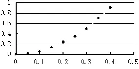
The data of knee joint angle changing with time is shown in Table 7.

Table 7: The data of knee joint angle changing with time

Time(s) 0.0 0.05 0.10 0.15 0.20 0.25 0.30 0.35 0.40

Angle(rad) 0.00 0.05 0.18 0.37 0.60 0.76 0.75 0.57 0.20

The change trend of the knee joint angle over time is shown in Figure 7.

Figure 7: The change trend of the knee joint angle over time

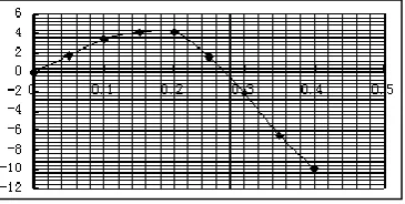
The data of knee joint angular velocity changing with time is shown in Table 8.

Table 8: The data of knee joint angular velocity changing with time

Time(s) 0.0 0.05 0.10 0.15 0.20 0.25 0.30 0.35 0.40 (rad/min) 0.00 1.75 3.42 4.13 4.18 1.61 -2.11 -6.51 -9.91

The change trend of the knee joint angular velocity over time is shown in Figure 8.

Figure 8: The change trend of the knee joint angular velocity over time

CONCLUSION

[image:7.595.213.403.355.457.2] [image:7.595.216.399.570.662.2]

(8)

data of knee joints and related systems in the starting process, and verifies the reliability of the model through the simulation results. This model established in this paper can simulate the movement situation of the knee over time, which is similar with the actual human movement and can be used as a mathematical model for simulation analysis.

REFERENCES

[1]Qian Jing-Guang. Journal of Nanjing Institute of Physical Education (Natural Science). 2006.5(1):01-05. [2]Bing Zhang,Yan Feng, 2013, International Journal of Applied Mathematics and Statistics, 40(10), 136-143. [3]Cai Xin. Journal Of Henan Normal University(Natural Science). 2010.38(4):167-169.

[4]Liu Hui. Mechanics in Engineering. 2005.27(2):63-66.

[5]Wang Xi-Shi, Bai Rui-Pu. Advances In Mechanics.1999.29(2):244-250. [6]Feng Guang-Ming. Journal Of Biomedical Engineering.2005.22(1):189-192. [7]Zhou Yuan-Hua. Computer Applications And Software.2004.21(1):57-60.

[8]Zhang Yue-Jin, Song Jian. Mechanical Science and Technology.1997. 16(5):753-759.