All Pairs Shortest Paths Algorithm for High dimensional Sparse Graphs

All-Pairs Shortest Paths Algorithm

for High-dimensional Sparse Graphs

Urakov A. R.

,

Timeryaev T. V.

∗

General Scientific Faculty, Ufa State Aviation Technical University, Ufa, 450077, Bashkortostan, Russia

∗_{Corresponding Author: [email protected]}

Copyright c⃝2013 Horizon Research Publishing All rights reserved.

Abstract

Here the All-pairs shortest path prob-lem on weighted undirected sparse graphs is being considered. For the problem considered, we propose “disassembly and assembly of a graph” algorithm which uses a solution of the problem on a small-dimensional graph to obtain the solution for the given graph. The proposed algorithm has been compared to one of the fastest classic algorithms on data from an open public source.

Keywords

APSP, graph disassembly, graph assem-bly, graph contraction, sparse graphs

1

Introduction

The APSP (all-pairs shortest path problem) is one of the most popular tasks in graph theory because the shortest paths between all pairs of vertices are used for solving many problems involving discrete optimization (TSP, theory of transportation task etc). Moreover, the task itself is of great interest in research.

Recently this problem has gained new interest due to a growing number of highly detailed graphs that are gen-erated automatically and describe structures from the real world. Such graphs have about 106_{or more vertices}

and this number will inevitably increase. So the accel-eration of APSP solving for high-dimensional graphs is becoming highly important.

Because of its popularity, there are a lot of APSP solution algorithms but there isn’t any method to obtain the solution as fast for different kinds of input data. That’s why APSP solution algorithms can be classified according to the type of graph as follows: directed [3], complete [5], weighted [4], unweighted [1] and sparse [7]. Here we present an algorithm for solving the APSP for weighted, undirected and high-dimensional sparse graphs with non-negative weights.

This paper is organized as follows. In section 2, we introduce notation and the problem definition, in section 3, we describe the algorithm and in section 4 we show the results in comparison with one of the most renowned APSP algorithms.

2

Notation and problem

defini-tion

2.1

Terms and definitions

Here, we consider a connected, undirected and sparse graph G = (V, E, w), where each edge e(vi, vj) has a

non-negative weight w(i, j). The given graph Gis con-sidered to be simple (has no loops or multiple edges).

Denote by|V|=nthe order of a graphor cardinality of vertices set. Denote by |E|=m the size of a graph or cardinality of edges set.

Denote byw(i, j)the weight of the edge between ver-ticesviandvj(w(i, j) =∞, for non-connected vertices).

A degree d(vi) of vertexvi is the number of edges

inci-dental tovi. A graph is calledsparse ifm≪n2.

A path is an alternating sequence of vertices and edges

v0, e1,v1, . . .,vk₋1,ek,vk, beginning and ending with

a vertex. In that sequence, each vertex is incidental to both the edge that precedes it and the edge that fol-lows it. A length of a path is the sum of the weights of its edges. A distance m(i, j) between vi and vj is

the length of the shortest path ps_ij =ps(vi, vj) between

these vertices. A distance matrix is a matrix in which each element at the intersection ofith row and jth col-umn contains the length of the shortest path between

vi andvj. A graph is said to beconnected if every pair

of vertices in the graph is connected by some path, i.e.

mij<∞, ∀i, j.

Between any pair of vertices there can be more than one shortest path. We do not consider it as an essential issue in this paper, so the references to the shortest path can mean any of them.

A matrix is calleda precedence matrix if each element

pij of the matrix corresponds to the vertex that

pre-cedes vertexvj in the path fromvito vj. Therefore the

elements of P can be determined by

pij = {

vk, ∃vk:psij =. . . vk, e(vk, vj), vj

∞, else Using P the shortest path ps

ij from vi to vj in a

con-nected graph can be obtained by the recursive formula:

ps_ij=

{

ps_(v

i, pij), e(pij, vj), vj, pij ̸=vi

Now, we shall give the following supplementary definitions. Let us call a graph sequence S =

{G1, G2, . . . , Gr} shrinking graph G0 = (V0, E0, w0),

where Gp = (Vp, Ep, wp), Vp = {

v₁p, vp₂, . . . , vp_n(p)

}

,

Ep = {

ep₁, ep₂, . . . , ep_m(p)

}

: ep_i = ep(v_jp, vp_k) ⊆ Vp×Vp

andwp:Ep→[0,∞).

Every next graph Gp+1 of the sequence is obtained

from the previous Gp by the removing the k vertices

and the edges incidental to them, plus the addition of new edges and by recalculating the weights of the edges adjacent to the deleted ones.

For these graphs, we get|Vp|>|Vp+1|,∀p= 0, r−1.

Denote byv_ip+1a vertex ofGp+1corresponding to vertex

v_ipofGp. Denote byep+1 (

vp_j+1, v_kp+1

)

an edge of Gp+1

corresponding to the edgeep(_vp j, v

p k )

ofGp.

Denote by Gp+1 = Rp(v p

1, v

p

2, . . . , v

p

k) the graph

ob-tained from Gp by removing the vertices vp1, v

p

2, . . . , v

p k

and the edges incidental to them. For this graph we get

wp+1(i, j) =wp(i, j),∀i, j:vip+1, v

p+1

j ∈Vp+1.

Denote bymp_{(i, j) the distance betweenv}p

i andv

p

j in

Gp. ByMp = (

mp_ij)denote the distance matrix of Gp.

Also denote byvp_i

l lth adjacent tov

p

i vertex and byA p i

the set of all adjacent tovp_i vertices in graphGp.

2.2

Problem definition

Given a connected, undirected, simple, weighted and sparse graphG= (V, E, w), where each edge has a non-negative weightw:E→[0,∞). Find the shortest paths between every pair of vertices of the graph, i.e. find the distance matrixM and the precedence matrix P of the graph.

3

Algorithm of the solution

3.1

Main idea

The main idea of the introduced algorithm is to reduce the problem on a large graph to the problem on a smaller graph. The algorithm can be partitioned into 3 stages.

1. Compression. A large initial graph is replaced by a small graph.

2. Microsolution. The APSP for the small graph is solved by using any known method.

3. Restoring. The APSP solution for the small graph is projected onto the initial graph.

While using this method we must satisfy the following conditions: a) validity ”—the compression must keep information about the shortest paths of the initial graph; b) efficiency ”—the introduced method must be quicker than all others.

The algorithm in which similar ideas were used are considered in [6]. Here we introduce an algorithm of a graph disassembly/assembly for large sparse graphs. At the disassembly stage, we consistently remove vertices, and then solve the APSP for the resulting small graph. At the assembly stage the initial graph is restored with the calculation of distances and paths.

3.2

Disassembly

The disassembly stage consists of consistent approx-imation of the initial graph G0 = (V0, E0, w0) by the

graphs of a shrinking sequence S = {G1, G2, . . . , Gr}.

Here we consider a particular case in which every next graph Gp+1 of the sequence S is obtained by removing

only one vertex fromGp.

Suppose that vertex vp_i is to be removed. Let the de-gree ofv_ipbe equal tok. If any shortest path containsv_ip

(except shortest path straight to or from vp_i) then this path contains subpathv_ip_j, ep(v_ip_j, vp_i), vp_i, ep(vp_i, v_ip_l), v_ip_l :

j, l∈ {1,2, . . . , k}. Therefore to remove vertexv_ip prop-erly, we need to preserve the shortest paths only between vertices adjacent tovp_i.

By wpmv(1,2,...,h)(ij, il) =

ming=1,2,...,h(wp(ij, g) +wp(g, il)) denote the

min-imum sum of the weights of two edges which connect vertices v_ip_j, v_ip_l and are incidental to a common vertex that belongs to the setvp₁, v₂p, . . . , v_hp ofGp. To preserve

distances it is sufficient to have

wp+1(ij, il) =       

min

(

wpmv(i)(ij, il), wp(ij, il) )

,

ifwpmv(i)(ij, il)< w

mv(h_̸=i)

p (ij, il)

wp(ij, il),else

(1) for any pair

(

v_ip

j, v

p il

)

inGp+1.

At the beginning of the algorithm any element of

P′ is equal to infinity p′_ij = ∞, ∀i, j. To pre-serve the information about the shortest paths, for each element of P′ that satisfies wmv(p i)(ij, il) <

min

(

wp(ij, il), w

mv(h_̸=i)

p (ij, il)

)

we have

p′_ijil=

{

vi, p

′

iil=∞

p′_ii

l, p ′

iil̸=∞

(2)

Note: if vertexv_ip, which is to be removed, is adjacent only to one vertex of Gp, so, as there are no shortest

paths passing through v_ip, the vertex and the inciden-tal edge are simply removed without the shortest path preservation.

We use three parameters for the disassembly stage.

dmax ”—is the maximum degree of the vertices to be

removed. nmin”—is the order of graphGr, which is the

last (smallest) graph of the shrinking sequence. Imax

”—is the limit of the increasing number of edges after the removal of one vertex. The assignment of values to

dmax, nmin and Imax is a problem in itself, which will

be discussed elsewhere. The results, which are shown in part 4, have been obtained by assignment dmax =

Imax=∞,nmin= 1.

Let us try to remove vertex vp_i with all of its k inci-dental edges and preserve the shortest paths. Denote by

I(v_ip) =

        

I(v_ip) + 1,

ifwp(ij, il) =∞

∧ wpmv(i)(ij, il)< w

mv(h̸=i)

p (ij, il)

I(v_ip),else

(3)

Thus we’ll obtain the change in the size of graphGp+1

relative toGp after the removal of vertexvpi. IfI(v p i)>

0, then the graph size increases, otherwise the graph size decreases or remains the same. Using (3) we expect that the increase of the graph size is bounded above byImax

when a vertex is removed. It follows that vertexvp_i can be removed only ifI(vp_i)≤Imax.

The selection of the vertices that we are going to re-move is performed in the following way. Since vertices meeting d(v_ip) < 3 can be removed anyway, it follows that vertices should be removed in ascending order of their degrees from 1 to dmax. This speeds up the

al-gorithm due to a smaller number of processed vertices with degrees close todmax. After we removev

p

i, the

de-grees of the adjacent vertices can change, hence, if we remove v_ip, the vertices adjacent to vp_i should be pro-cessed through recursion. The graph disassembly algo-rithm and an auxiliary algoalgo-rithm of vertices inspection and removal are on fig. 1 and 2.

Vertices inspection and removal

Input: vertexv_ip, number of verticesnc,Imax,dmax,

nmin,p, P

′

.

Step 1. Vertices inspection Ifd(v_ip)<3, go to step 2.

ElseI(vp_i) =−d(v_ip). Inspect all pair of verticesAp_i and changeI(vp_i) by (3).

IfI(vp_i)≤Imax, go to step 2.

Else end of algorithm. Step 2. Vertex removal

Form a new graphGp+1=Rp(vip).

Count the weights of the edges between verticesAp_i by (1).

Change the elements of the matrixP′ by (2).

nc=nc−1,t=p,p=p+ 1.

Ifnc=nmin, end of algorithm.

Else, whilenc> nmin for verticesv p il:d

(

v_ip

l

)

< d(vt

il

)

do Vertices inspection and removal (vp_i

l, nc, Imax, dmin, nmin, p, P ′

[image:3.595.298.552.51.283.2]

).

Fig. 1: Auxiliary algorithm of vertices inspection and removal.

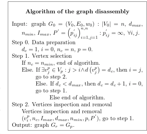
Algorithm of the graph disassembly

Input: graph G0 = (V0, E0, w0) : |V0| = n, dmax,

nmin,Imax, P

′

=

(

p′_ij

)n,n

i=1,j=1:p

′

ij =∞, ∀i, j.

Step 0. Data preparation

dc= 1, i= 0,nc =n,p= 0.

Step 1. Vertex selection

Ifnc=nmin, end of algorithm.

Else. If∃vp_j ∈Vp:j > i∧d (

v_jp)=dc, theni=j,

go to step 2.

Else. Ifdc < dmax, thendc=dc+ 1,i= 0,

go to step 1.

Else end of algorithm. Step 2. Vertices inspection and removal

Vertices inspection and removal (v_ip, nc, Imax, dmax, nmin, p, P

′

), go to step 1. Output: graphGr=Gp.

Fig. 2: Algorithm of the graph disassembly.

3.3

Microsolution

Here the APSP for Gr is solved. The result of the

stage is the distance matrix Mr of Gr. We use matrix

M_r′ =Mr and recalculateP

′

by

p′ij = {

pr

ij, p

′

ij=∞ ∧ p

′

pr ijj=∞

p′_pr ijj, p

′

ij=∞ ∧ p

′

pr ijj̸=∞

(4)

p′ij = {

pr

ij, wr(i, j)> mrij ∧ p

′

pr ijj =∞

p′_pr

ijj, wr(i, j)> m

r

ij ∧ p

′

pr ijj ̸=∞

(5)

here pr_ij are the elements of the matrix Pr = (

pr_ij), which corresponds toGr. The calculated paths are the

shortest ones due to the usage of the distances preser-vation method. In other words, we have m′r

ij =mrij =

m0

ij,∀i, j:vri, vrj ∈Vr.

Obviously, ifGrhas only one vertex then this stage is

skipped and the assembly of the graph starts.

3.4

Assembly

Before this stage starts, the graph assembly sequence

S ={G0, G1, . . . , Gr} is defined. HereG0 ”—is the

ini-tial graph, Gr ”—is the smallest graph. The shortest

paths between all vertices ofGrwere found in the

previ-ous stage. At the assembly stage we restore the removed vertices in reverse order to their removal. That is we move fromGrtoG0throughGr−1, Gr−2, . . . , G1,

recal-culating the shortest paths for vertex v_ir−p : v_ir−p+1 ∈/ Vr−p+1∧v

r₋p

i ∈Vr−p in each stepp.

Suppose vertex vr_i−1 is to be restored, i.e. we move from Gr to Gr₋1. Vertex vir−1 is connected with

ver-tices {v_ir_z−1}k_z=1 by k edges. Matrix Mr′ = Mr of

Gr was found in the previous step, therefore to find

the matrix M_r′₋₁ of Gr−1, we only need to calculate

the shortest paths from vertex v_ir−1 to all other ver-tices of Gr−1. Other elements of M

′

r−1 are assigned

equally to the corresponding elements of M_r′, that is

m′_jlr−1=m′r

jl,∀j, l:v r

[image:3.595.62.298.445.718.2]

[image:4.595.64.537.65.542.2]

Table 1. Characteristics of graphs used for testing

Group Avg. quantity of Avg. quantity of Average Max

Graphs graphs Vertices Edges vertex degree vertex degree

G1 103 _2,5·103 _{2,48 6}

10

G2 2·103 _5,21·103 _{2,6 5}

G3 3·103 _7,88·103 _{2,62 6}

G4 4·103 1,07·104 2,68 6

G5 5·103 _1,33·104 _{2,66 6}

G6 6·103 _1,58·104 _{2,63 7}

G7 7·103 _1,85·104 _{2,64 6}

G8 8·103 2,08·104 2,6 6

G9 9·103 _2,36·104 _{2,62 7}

G10 104 _2,72·104 _{2,72 7}

GR 2,1·103 _6·103 _{2,86 14 20}

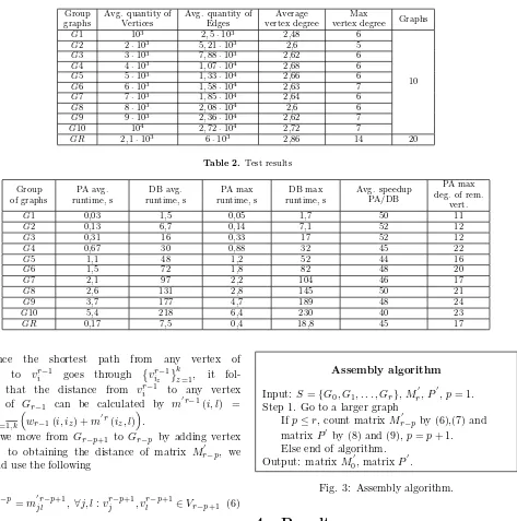
Table 2. Test results

Group of graphs

PA avg. runtime, s

DB avg. runtime, s

PA max runtime, s

DB max runtime, s

Avg. speedup PA/DB

PA max deg. of rem.

vert.

G1 0,03 1,5 0,05 1,7 50 11

G2 0,13 6,7 0,14 7,1 52 12

G3 0,31 16 0,33 17 52 12

G4 0,67 30 0,88 32 45 22

G5 1,1 48 1,2 52 44 16

G6 1,5 72 1,8 82 48 20

G7 2,1 97 2,2 104 46 17

G8 2,6 131 2,8 145 50 21

G9 3,7 177 4,7 189 48 24

G10 5,4 218 6,4 230 40 23

GR 0,17 7,5 0,4 18,8 45 17

Since the shortest path from any vertex of

Gr−1 to vri−1 goes through {

v_ir−1

z

}k

z=1, it

fol-lows that the distance from v_ir−1 to any vertex

v_lr−1 of Gr₋1 can be calculated by m

′_r−1

(i, l) = min_z=1,k

(

wr−1(i, iz) +m

′_r

(iz, l) )

.

If we move from Gr−p+1 to Gr−p by adding vertex

v_ir−p, to obtaining the distance of matrix Mr′₋p, we

should use the following

m_jl′r−p=m_jl′r−p+1, ∀j, l:v_jr−p+1, v_lr−p+1∈Vr−p+1 (6)

m′_ilr−p=m′_lir−p= min_z=1,k

(

wr−p(i, iz) +m

′_r−p+1

(iz, l) )

,

∀l:v_lr−p+1∈Vr−p+1

(7)

Denote by x(l) the number iz such that x(l) :

wr−p(i, x(l)) +m

′_r−p+1

(x(l), l) = min_z=1,k

(

wr−p(i, iz)m

′_r−p+1

(iz, l) )

. If any vertex sat-isfies wr−p(i, l) > m

′_r−p

il ∨ wr−p(l, i) > m

′_r−p

li or

p′_il = ∞ ∨ p′_li = ∞, then the respective elements of matrixP′ should be changed by

p′_il=

{

vi, p

′

x(l)l=∞

p′_x(l)l, p′_x(l)l̸=∞ (8)

p′_li=

{

vl, p

′

x(l)i=∞

p′_x(l)i, p′_x(l)i̸=∞ (9) The assembly algorithm is shown in Figure 3.

Assembly algorithm

Input: S ={G0, G1, . . . , Gr}, M

′

r,P

′

,p= 1. Step 1. Go to a larger graph

Ifp≤r, count matrixM_r′_−p by (6),(7) and matrixP′ by (8) and (9),p=p+ 1. Else end of algorithm.

Output: matrixM0′, matrixP

′

.

Fig. 3: Assembly algorithm.

4

Results

All the tests have been performed on a computer equipped with an Intel Core 2 Duo E8400 (3 GHz) CPU and 2 GBs of RAM on the 32-bit edition of Windows XP. The source code has been written on C++ programming language in Borland C++ Builder 6. Weighted graphs of the USA road networks from an open public source (G1−G10) [8] have been used as the test data. Con-nected subgraphs with sizes from 103_{to 10}4_{of 10 pieces}

for each size have been derived from graphs G1−G10. Another set of test data are the graphs of Russian cities’ road networks ((GR, for detailed specifications look at [2]). The details of the test graphs are shown in Table 1.

Test parameters are dmax = Imax = ∞, nmin = 1.

[image:4.595.107.218.718.788.2]

The proposed algorithm speeds up the solving of APSP an average of 47 times faster in comparison with the Dijkstra algorithm. For each and all test graphs the algorithm is faster than the Dijkstra’s algorithm (the minimum speed up is 34 times faster). During the tests, the vertices degrees were increased to a maximum of 17. This means that the complexity of the vertices removal increases during the disassembly only slightly.

5

Conclusion

The proposed algorithm noticeably accelerates the solving of the APSP for graphs of road networks, which is confirmed by the tests. The objects of further research may be the selection of the algorithm parameters based on a fast analysis of graph properties, the modification of the disassembly and assembly order and the scalabil-ity issues of the algorithm relative to the increasing of a graphs’ dimensions. Also, it is interesting to modify the algorithm to solve the problem quicker, but within a given error.

REFERENCES

[1] T. H. Cormen, C. E. Leiserson, R. L. Rivest, C. Stein. Introduction to algorithms. 2nd ed., MIT Press, Cambridge, 2001.

[2] A. R. Urakov, T. V. Timeryaev. Using weighted graphs features for fast searching their parameters, Prikl. Diskr. Mat., No.2, 95-99, 2012.

[3] R. Bellman. On a Routing Problem, Quarterly of Applied Mathematics, No.16, 87-90, 1958.

[4] E. W. Dijkstra. A Note on Two Problems in Connex-ion With Graphs, Numerische Mathematik, No.16, 269-271, 1959.

[5] R. W. Floyd. Algorithm 97: Shortest Path, Communi-cations of the ACM, No.5(6), 345, 1962.

[6] R. Geisberger, P. Sanders, D. Schultes, D. Delling. Contraction Hierarchies: Faster and Simpler Hierarchi-cal Routing in Road Networks, International Workshop on Experimental Algorithms (WEA 2008), 319-333, 2008.

[7] D. B. Johnson. Efficient algorithms for shortest paths in sparse graph, Journal of the ACM, Vol.24, No.1, 1-13, 1977.

[8] 9th DIMACS Implementation Challenge,

”—Shortest Paths, Online available from