Cycling in Newton’s Method
Mikheev Serge E.
Faculty of Applied Mathematics & Control Processes,Saint Petersburg State University, 198504, Russia
∗Corresponding Author: [email protected]
Copyright c⃝2013 Horizon Research Publishing All rights reserved.
Abstract
Cycling in Newton’s method for systems of nonlinear equations in multi-dimensional spaces is researched. The functions of the system have most favorable for convergence properties such as convexity or concavity, no singularity of Jacobi’s matrix for the functions and of course existence of the root. It was shown by the counterexample that these properties does not prevent cycling in pure Newton’s method while various relaxations of the method have good convergence.Keywords
cycling, cycle, convergence, nonlinear equation, iteration1
Introduction
Let us consider a system of linear equations
g(x) = 0, (1)
g:Rn −→Rn. One of the common methods of obtain-ing iterative approximations to a solution α of (1) (in other words: αis a root ofg) is the Newton’s one (NM) xk+1=xk−J−1(xk)g(xk), k= 1,2, ... (2) where J is Jacobi’s matrix of function g. Equally pop-ular is the simplified Newton’s method (SNM), which in contrast to the main method uses the initial matrix J(x0) instead of J(xk) for each iteration.
The choice of initial approximationx0lies outside NM and SNM.
In contrast to scalar case the problem of NM con-vergence in multidimensional one was waiting its hour till 1948. Then Kantorovich has published the theorem about semiglobal convergence of NM and SNM in Ba-nach’ spaces. After a short space several close to the theorem results were discovered by Kantorovich himself and his disciple Mysovskikh. The results are presented in [1]. To better understand what problems in NM were left to other researchers we use some other language to describe the results.
There is a key condition in Kantorovich’ and Mysovskikh’ theorems. If one extracts it then the re-maining ones can be regarding as forming a class of func-tions. Such a class for Kantorovich’ theorem [1, p. 680]
is a set of functionsgdefined in some ball centered in ini-tial point x0, J must have derivativeJ′ in the ball and
in the point x0 the continuous linear operator J−1(x0)
exists, such that ∥J−1(x0)J′(x)∥ ≤K in the ball. So,
the class may be denoted as K(x0, J(x0), K). The key
condition of the theorem isK∥J−1(x0)g(x0)∥ ≤1/2. It provides convergence both NM and SNM for each ele-ment of class K(x0, J(x0), K). As the class K and the key condition contain no estimation of ∥α−x0∥ the theorem is not local. From the other hand the key condi-tion contains discrepancy, butKcontains elements with arbitrary large discrepancy, so, the key condition is not valid for whole K. This means that the theorem is not global for K. So, the theorem is semiglobal. Neverthe-less practice needs demanded more.
At first, it is hard to obtain and to use a second deriva-tive in multidimensional case. Therefore having lost very little in the power of the theorem, the class K was en-riched up to the class K+ by functions with derivatives
satisfying Lipschitz’ condition with constant L. Then the theorem takes the form ‘ifg∈ K+(x0,∥J−1(x0)∥, L)
and the key condition L∥J−1(x0)∥2∥g(x0)∥ ≤ 1/2 is
valid then for each element of K+(x0,∥J(x0)∥, L) both
NM and SNM generate sequences convergating toα’. At second, even after a big work to estimate parame-ters K or Lof these classes it is necessary to calculate g(x0), J−1(x0) and only to know is the convergence
guaranteed or may be here is a chance of divergence. Partly the reason, partly real equations pushed to new classes. For example, Mysovskikh examined the class
M(x0, B, L) where B≥ ∥J−1(x)∥for all xin the ball. He has proved the convergence of NM for elements of
M satisfying the key condition LB2∥g(x0)∥ < 2. So,
only the discrepancy should be calculated. Quite an-other classes where NM and SNM can convergate are proposed in [2]. But the convergence in it is supported also only by local and semiglobal theorems.
Besides practice needs there are additional incentive to find classes with global convergence of the methods. This is the simplicity of global convergence in the scalar case. It was well known yet to Newton that the global convergence in the scalar case both NM and SNM can be provided by
1) condition for method validity SNM: existence ofg′(x0) andg′(x0)̸= 0;
NM: (∀x)∃g′(x)̸= 0;
NM & SNM: rootαexists, gis convex or concave; SNM: x0 must satisfy g(x0)≥0 under convexity and g(x0)≤0 under concavity.
Another incentive is simplicity of global result for modification of the methods by various relaxations, par-ticularly by their limit, when relaxation step tends to zero, version which is finding rootαas a solution of the Cauchy’ problem ˙x=J−1(x)g(x), x(0) =x0. Gavurin
[3] has found conditions for existence of a limit point ¯
x= limt→∞x(t) of the solution be a root α. He has formulated his result by such a way that it has become local. Strengthening one condition and omitting another in Gavurin’s theorem we can get the same affirmation for each initial pointx0 in Banach’ spaceB, i.e. global result. Namely, let 1) (∀x∈B)∥J−1(x)∥ ≤γ; 2)J′(x) is bounded in a neighborhood of each xin B. Then ¯x exists and equals toα.
Despite various relaxations with positive steps were also very fruitful for global results (e.g. [4]) the interest to pure NM and SNM did not die.
The global convergence inRnfor convex functions g
is set [5] when J−1(x)≥0 for allx, where the
inequal-ity is understood componentwise. In general case, the elucidation of such a positivity of J−1 is very difficult.
Checking the conditions of the theorems of semiglobal convergence is somewhat simpler, but the results are only permissions to use NM and SNM from specific ini-tial point, that significantly reduces the theoretical value of the theorems. And a numerical experiment often re-quires significantly less human efforts than checking the conditions of the convergence theorems. Therefore most of the applications of NM and SNM in the multidimen-sional case is blindfold ‘i.e. without prior analysis of the initial point for the convergence from it’. Therefore, the following question seems to be of the practical interest: does only easy checking convexity of g with the condi-tion of non-singularity of the Jacobi’s matrix throughout the multidimensional space guarantee convergence, as in the one-dimensional case?
The analysis of the next example shows that it is, unfortunately, wrong already in R2 and even when J satisfies Lipschitz’ condition.
2
Methodology
Here we name a reflection to finite-dimensional space convex when all its components are convex.
Counterexample(of bad convex reflection). Let g: R2→R2, g(x) = (g1(x), g2(x)).
We defineg1 andg2 via their graphs, which are
con-structed as convex slope cylindrical surfaces. Then for each functions the level lines defined by the equations g1(x) = 0, g2(x) = 0, can be interpreted as
guid-ing lines in the plane of the arguments. We construct each of them as combinations of pairs of convex parabo-las and pair of rays with smooth connections in points
y= 0,±τ. Let x= (y, z), t0>0, L > l >0 and
0 =h1(x) :=
ly2+t
0y−z, 0≤y ≤τ,
Ly2+t
0y−z, 0> y ≥ −τ,
(2lτ +t0)y−lτ2−z, y > τ,
(−2Lτ+t0)y−Lτ2−z, y <−τ;
(3)
0 =h2(x) :=
ly2−t0y−z, 0≤y ≤ −τ,
Ly2−t
0y−z, 0< y ≤τ,
(−2lτ −t0)y−lτ2−z, y <−τ.
(2Lτ−t0)y−Lτ2−z, y > τ,
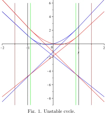
[image:2.595.300.540.56.237.2](4) It is evident thatg has a single root α= (0,0).
Fig. 1 shows the guiding lines under t0= 1, τ = 1,
L = 2.25, l= 1.5. Here the curve (3) is blue and the curve (4) is red.
Fig. 1. Unstable cycle.
We rout the forming lines of the cylindrical surfaces so that their projections on the plane of arguments (y, z) are parallel to the axis of symmetry i.e. axis z and the surfaces become convex. The forming lines slopes of both graphs are identical and from interval (0◦,90◦).
In other words g1(x) =wh1(x), g2(x) =wh2(x) and
w∈(0,+∞). We shall be quite satisfied with w= 1. Each step of Newton’s method has a simple geometric interpretation in the plane of x= (y, z). Through the current iteration xk = (yk, zk) a straight line is drawn parallel to the axis of symmetry. At its intersections with lines of levels g1(x) = 0, g2(x) = 0 in points
(yk, z
1(yk)) and (yk, z2(yk)), tangents to these lines
are drawn. The intersection of the tangents is the next iteration xk+1. The second coordinatezk of the current iteration is not involved in the actions.
On Fig. 1 the tangents of both steps have the colors of their curves. Each point on the right green vertical (y= b
[image:2.595.310.530.289.524.2]left branches of curves (3) and (4) in the points with abscissa of left green vertical is the third iteration lying on the right green vertical. These two intersections of the tangents are the points of the single unstable cycle on two points. Outside the strip bounded by two black verticals (y =±1) the functiong is linear. ( See 3.1.) Extremely left and extremely right brown verticals have abscissas of two point stable cycle (y=±1.5).
3
Results
3.1
CyclesLet us define the relationship between the first co-ordinates y and v of two successive iterations, when 0< y < τ. Following geometric interpretation, we con-sider the equations of the tangents to the lines of levels:
z=t1(y)(v−y) +z1(y),
z=t2(y)(v−y) +z2(y).
(5)
Here t1, t2 are tangents of slope angles of tangents to
the lines of levels. Differentiating the expressions (3) and (4) yields them:
t1(y) = 2ly+t0, t2(y) = 2Ly−t0, (6)
where z1, z2are implicit functions defined by equations
(3) and (4), respectively:
z1(y) =ly2+t0y, z2(y) =Ly2−t0y. (7)
Substituting (6), (7) in (5) and excluding z give the equation for the first coordinatev of the next iteration: (2ly+t0)(v−y)+ly2+t0y= (2Ly−t0)(v−y)+Ly2−t0y
or
(2ly+t0)v−ly2= (2Ly−t0)v−Ly2.
Hence v y =
(L−l)y 2[(L−l)y−t0]
= 1
2−2τ0/y
. (8)
Here we introduced the principal parameter τ0:=t0/(L−l).
Its geometric sense is the abscissa of the point where two right wings parabolas have parallel tangents.
When the y takes values [0, t0/(L−l)), the
nu-merator continuously increases monotonically from zero. The negative denominator also grows continuously and monotonically to zero. Consequently, the right side of (8) takes in reverse order all the values of the semiaxis (−∞,0]. If
y=by=. 2t0 3(L−l) ≡
2
3 τ0 (9)
the right side is equal to−1. If 0> y≥ −τ we have v
y =
(l−L)y 2[(l−L)y−t0]
= 1
2 + 2τ0/y
(10) which with y := −by also yields v/y = −1. Thus, with choice y0=±yb and τ≥yb Newton’s method for
system (g1(x), g2(x)) = (0,0) has a cycle at two points
with abscissas ±by and with a single ordinatebz. Under (5), (6), (7)
b
z=t1(y)(b −2y) +b z1(y) =b −3lby2−t0by=−
2t2 0
3
L+l (L−l)2.
Obviously, from (8), (10) by the same way we prove convergence of Newton’s method when
0<|y0|<by ∧ |y0|< τ,
and iterations removal from α, when τ ≥ |y0| > y.b
Consequently, when τ > yb aforementioned cycle can be characterized as unstable and it has practically no chances to be realized on a computer, because the cal-culation errors will most likely push out from the cycle the iterations to the domain of convergence or diver-gence. The chances of a cycling under τ =yb and the choice of |y0| ≥yb are also small but much more real.
If τ∈(by, τ0), then at a distance greater thanτ from
the axis of symmetry, additionally, there is a stable cycle at two points.
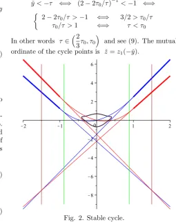
Really. All the cases with positive y ≤τ are con-sidered yet. Let y > τ. Then to determinev we can continue rays 3 from (3) and 4 from (4) to their inter-section (see Fig. 2).
(2lτ +t0)v−lτ2= (2Lτ−t0)v−Lτ2.
This implies
v= ˇy:= (L−l)τ
2
2[(L−l)τ−t0] ≡
(
2−2τ0/τ
)−1
τ.
It is clear that inequality ˇy <−τis a sufficient condition to exist cycle on two points with abscissas ±y. Butˇ
ˇ
y <−τ ⇐⇒ (2−2τ0/τ)− 1
<−1 ⇐⇒ {
2−2τ0/τ >−1 ⇐⇒ 3/2> τ0/τ
τ0/τ >1 ⇐⇒ τ < τ0
In other words τ∈ (2
3τ0, τ0 )
[image:3.595.295.551.461.784.2]and see (9). The mutual ordinate of the cycle points is ˇz=z1(−y).ˇ
Fig. 2. Stable cycle.
g then the second iteration is one of the cycle points. That implies its stability. Moreover, (8) implies mono-tone increase of |v(y)| whenyruns (by,1). This means that NM starting with y ∈ y,b 1) will put out itera-tions moving away from ordinate axis with increasing rate. So, NM’ iteration reach the linearity domain for a finite number of steps. Therefore the two point cycle on (±y,ˇ z) attracts NM’ iteration if and only if abscissaˇ y of initial iteration satisfies |y|>y.ˇ
In Fig. 1 the domain of attraction to the stable cycle points is a part of plane outside the strip between two green lines.
3.2
Newton’s method correctness researchIn one-dimensional space for global convergence of Newton’s method with a convex functiongit is sufficient to require the possibility of constructing a Newtonian it-eration in all points in space, i.e. g′(x)̸= 0, ∀x∈R1.
In the counterexample with convex functions the finite decision obviously exists. Hence foresaid part 2) of suf-ficient conditions for convergency of NM in scalar case continues to be valid. But can NM be non applicable to the function g built in this counterexample in some points of spaceR2?
We have found the condition of NM’ correctness for counterexample.
Theorem. Let Newton’s method be applied to the vector-function g=h,hgiven by the formulas(3), (4). Then the condition τ < τ0 :=
t0
L−l is necessary and
sufficient for the method to be correctly defined in the whole spaceR2.
Proof. Necessity. If τ ≥τ0, for x= (τ0, z) one
must use the first case of (3) and the second one of (4). Then
∇g1(x)|x=(τ0,z)= (2lτ0+t0,−1)≡
≡(2Lτ0+t0,−1) =∇g2(x)
x=(τ0,z)
∀z.
Consequently, Jacobi’s matrix of g is singular in the pointxand NM is not applicable.
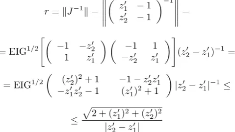
Sufficiency. We estimate from above the norm of ma-trix inverse to Jacobi’s one. Gradient ∇g1(x),
de-pending only on the first coordinate y, is (z′1(y),−1), function z1(y) implicitly defined in (3) (look (7)).
Similarly, ∇g2(x) = (z2′(y)),−1). Consequently,
r≡ ∥J−1∥= (
z1′ −1
z2′ −1 )−1
=
= EIG1/2 [(
−1 −z2′ 1 z1′
) (
−1 1
−z2′ z′1 )]
(z2′ −z1′)−1=
= EIG1/2 (
(z2′)2+ 1 −1−z2′z1′
−z1′z′2−1 (z1′)2+ 1 )
|z2′ −z′1|−1≤
≤
√
2 + (z1′)2+ (z′ 2)2
|z2′ −z1′|
Here EIG is the function which gets out the largest eigen-value of its matrix argument.
Obviously, the modulus of the tangents difference, which is the denominator, is constant in all points
y of the set {(−∞,−τ],[τ,+∞)} and is equal to
|2t0−2τ(L−l)|. The numerator reaches the global
maximum either at y= 0, or at y=τ.
Indeed, on the set [0, τ] the expression under the radical is a polynomial ofy:
P(y) := 2 + (t0+ 2ly)2+ (t0−2Ly)2≡
≡2 + 2t20−4(L−l)t0y+ 4(L2+l2)y2.
It has a positive coefficient at the highest degree, so P reaches a maximum value µ > 0 either when y = τ, or when y = 0. Note that P(y) = P(τ) ∀y ≥ τ. Consequently, we can set r(x)≤ √µ/[2t0−2(L−l)τ].
Thus, if τ ∈ (2
3τ0, τ0 )
then Newton’s method for system g(x) = (0,0) is defined on allR2 and has two
cycles, one of which is stable. Being defined also on all R2under τ= 2t0
3(L−l), it has only one unstable cycle.
⋄
Note 1. The minimum value of radicand, which is said about in the proof of the theorem, achieved with y= L−l
2(L2+l2)=ymin. Because of the symmetry of the
square polynomial relative to its minimizers the condi-tion
τ <2ymin≡ (L−l)t0 L2+l2
ensures that maximum value is achieved on the segment [0, τ] with y= 0. Then µ= 2 + 2t2
0. ⋄
Note 2. It is easy to show that the Jacobian matrix of the functiongintroduced in the counterexample has Lip-schitz’ constant throughout theR2. Thus, the function g belongs to the class to which Kantorovich’s theorem on the convergence of Newton’s method is applicable [1]. Semiglobal restriction of the theorem on the collective parameter L∥J−1∥2∥g(x0)∥ ≤1/2 for the above found
cycle is significantly disrupted, and this is in accordance with world known impossibility to weaken conditions of Kantorovich’s theorem. As the object of this theorem is a class of functions, the theorem being applied to the counterexample guarantees convergency of NM in domain DK which is smaller than the mentioned above
[image:4.595.44.284.622.757.2]strip. ContainingDK contour PK(x) = 1/2 is drawn in
Fig. 2 by black. ⋄
Note 3. It is easy to verify that the simplified New-ton’s method ( xk+1 = xk−(∇g(x0))−1g(xk) ) has two cycles under the same parameters, each with a pair of points with the same abscissas but with different or-dinates.
Note 4. After small modifications this counterexample can be extended to the case of strictly convex functions.
4
Conclusion
properties easy for verification and close to convergence. As checking positivity of inverse Jacobi’s matrix J−1
proposed by Ortega is very difficult, it seems best way for application of NM is to enrich it by a kind of relax-ation or to use it with care being ready for cycling or divergence.
Collaterally, the counterexample under concrete pa-rameters shows a huge difference between the large real convergence domain and the small theoretical one, which follows from Kantorovich’ theorem.
REFERENCES
[1] Kantorovich L. V., Akilov G. P. Funkcional’nyi analiz (in Russian), Moscow, 1977.
[2] Miheev S. E. Convergence of Newton’s method in dif-ferent classes of functions (in Russian), Computational Technologies, Vol.10, No.3, 72-86, 2005.
[3] Gavurin M. K. Nonlinear functional equations and continuos analoguesof itarative methods (in Russian), Izvestia VUZov, No.5(6), 18-31, 1956.
[4] Mikheev S. E. Method of exact relaxations (in Russian). Computational technologies, Vol.11. No.6, 71-86, 2006.