Solutions to dilation equations

(1)

Solutions to Dilation Equations

David Malone

<[email protected]>

(2)

There was a maths thesis submitted and for just one degree was admitted.

I just won’t say don’t to the library’s wont; and of no other’s work it consisted.

Or, somewhat less anapæsticly∗:

• This has not previously been submitted as an exercise for a degree at this or any other University.

• This work is my own except where noted in the text.

• The library should lend or copy this work upon request.

David Malone (October 26, 2016).

∗_See

(3)

Summary

This thesis aims to explore part of the wonderful world of dilation equations. Dilation equations have a convoluted history, having reared their heads in various mathematical fields. One of the early appearances was in the construction of continuous but nowhere differentiable functions. More recently dilation equations have played a significant role in the study of subdivision schemes and in the construction of wavelets. The intention here is to study dilation equations as entities of interest in their own right, just as the similar subjects of differential and difference equations are often studied.

It will often be Lp₍

R) properties we are interested in and we will often use Fourier Analysis as a tool. This is probably due to the author’s original introduction to dilation equations through wavelets.

A short introduction to the subject of dilation equations is given in Chapter 1. The introduction is fleeting, but references to further material are given in the conclusion.

Chapter 2 considers the problem of finding all solutions of the equation which arises when the Fourier transform is applied to a dilation equation. Applying this result to the Haar dilation equation allows us first to catalogue theL2₍

R) solutions of this equation and then to produce some nice operator results regarding shift and dilation operators. We then consider the same problem in_Rn _{where, unfortunately, techniques using dilation equations}

are not as easy to apply. However, the operator results are retrieved using traditional multiplier techniques.

In Chapter 3 we attempt to do some hands-on calculations using the results of Chap-ter 2. We discover a simple ‘factorisation’ of the solutions of the Haar dilation equation. Using this factorisation we produce many solutions of the Haar dilation equation. We then examine how all these results might be applied to the solutions of other dilation equations. A technique which I have not seen exploited elsewhere is developed in Chapter 4. This technique examines a left-hand or right-hand ‘end’ of a dilation equation. It is initially developed to search for refinable characteristic functions and leads to a characterisation of refinable functions which are constant on intervals of the form [n, n+ 1). This left-hand end method is then applied successfully to the problem of 2- and 3-refinable functions and used to obtain bounds on smoothness and boundedness.

(4)

(5)

List of Figures

1.1 Daubechies’s D4 generating function. . . 3

2.1 For variousA the boundary of R and B−n_D ₍_n _{= 0}_,₁_{, . . .}_{). . . .} ₂₄

2.2 Various self-similar-affine tiles. . . 28

3.1 πˇ for the example. . . 34

3.2 πˇ∗χ[0,1) for the example. . . 36

3.3 Constructing a basis for solutions of the Haar equation. . . 40

4.1 The left-hand end of a dilation equation. . . 49

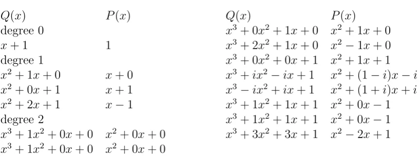
4.2 Checking a bit pattern to see if is it 2-refinable. . . 53

4.3 Possible values forQ(x) and P(x) from Mathematica. . . 55

4.4 How to generateP(x). . . 57

4.5 Possible coefficients . . . 62

4.6 The left-hand end of a dilation equation. . . 63

(8)

What are these things called Dilation

Equations?

1.1 Introduction

In this chapter we will try to get a basic feel for dilation equations. We will see how they arise in the construction of wavelets, investigate some examples and briefly outline some of the techniques used to analyse them.

1.2 Where do they come from?

A wavelet basis forL2₍

R) is an orthonormal basis of the form:

2−n2w(2nx−k) :k, n∈_Z .

The function w is usually referred to as the mother wavelet. In an effort to produce a theory which facilitated the construction and analyses of these bases, the notion of a

Multiresolution Analysis (MRA) was conceived.

Definition 1.1. A multiresolution analysis of L2(_R) is a collection of subsets {Vj}_j_∈_Z of

L2₍

R) such that: 1. ∃g ∈L2₍

R) so thatV0consists of all (finite) linear combinations of {g(·−k) :k ∈Z},

2. the g(· −k) are an orthonormal series in V0, 3. for any Vj we have f(·)∈Vj ⇐⇒ f(2·)∈Vj+1,

4. +∞

S

j=−∞

(9)

5. +∞

T

j=−∞

Vj ={0},

6. Vj ⊂Vj+1.

This structure can be viewed in an intuitive way. Consider trying to approximate some function f by choosing a function in V0. This amounts to choosing coefficients so that:

f(x)≈X

k

akg(x−k),

which is a common mathematical problem.

Now consider what happens when we move fromV0 toV1. This corresponds to allowing the choice of twice as many functions which are half as wide as before. This should result in a better approximation, and part 6 ensures that our choice of function in V1 can be at least as good as the choice in V0.

As we move along the chain Vn, we expect improving approximations off,

correspond-ing to improvcorrespond-ing resolution. Parts 4 and 5 ensure that these improvcorrespond-ing approximations converge in L2₍

R) and are not in some sense degenerate.

Once you have one of these MRA structures, there exist∗ recipes for constructing wavelets (eg. [33]). It is reasonably clear that the construction of the MRA rests heavily on locating a suitable g.

What can we say about g using Definition 1.1? Well, first V0 = span{g(· −k) :k ∈Z} so, using part 3 of the definition we know that V1 = span{g(2· −k) :k ∈Z}. Noting that

g ∈V0 ⊂V1 we conclude that:

g(x) =X

k

ckg(2x−k).

This equation, whereg(x) is expressed in terms of translates ofg(2x), is adilation equation

or two scale difference equation. A function satisfying such an equation is said to be

refinable, or to emphasise the scale: 2-refinable.

1.3 The Haar dilation equation

The Haar dilation equation is the most simple example which illuminates the structure of what is going on here. Consider χ[0,1), the characteristic function of the interval [0,1). Clearlyχ[0,1) =χ[0,1₂)+χ[1₂,1), however asχ[0,1₂)(x) =χ[0,1)(2x) andχ[1₂,1)(x) = χ[0,1)(2x−1) we see χ[0,1) is a solution of:

g(x) =g(2x) +g(2x−1).

(10)

[image:10.595.207.397.108.249.2]

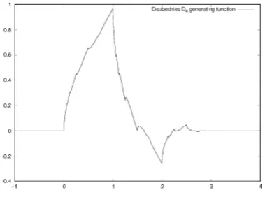
Figure 1.1: Daubechies’s D4 generating function.

This choice of g actually leads to a well-behaved MRA and in turn to the Haar wavelet basis of L2₍

R) given by the mother wavelet:

w(x) =



 

 

+1 if x∈[0,1₂)

−1 if x∈[1₂,1) 0 otherwise

.

This basis has been known since at least 1910. More recently, people have begun to pro-duce wavelet bases by solving carefully-chosen dilation equations with the aim of producing wavelets with particular properties. In particular in [9], Daubechies produces a whole fam-ily of orthonormal compactly-supported wavelets using this method. This famfam-ily, usually labeled D2N, uses 2N non-zero coefficients in the dilation equation to achieve smoothness

of roughly CN5. For small N, the functions are actually significantly smoother; Figure 1.1

showsD4 which is roughly 0.55 times differentiable.

1.4 Relating properties and coefficients

Some properties of g place simple conditions on the coefficients of the dilation equation. For example, if g is in L1(_R) and has non-zero mean, then integrating both sides of the dilation equation gives:

2 =X

k

ck.

Orthonormality of g(· −k) in L2(_R) can also be applied to give:

2δ0m =

X

k

ckck−2m,

(11)

The Strang-Fix condition, which tests for the ability to approximate xm, can also be used to give the condition:

0 =X

k

ck(−1)kkm.

These are the most common conditions imposed on coefficients in order to produce wavelets. So, given that we have chosen some set of coefficients, how do we go about finding a solution to the dilation equation with these coefficients? If it exists, will it be unique? Will it have the properties which we wanted?

1.5 Fourier techniques

Many of those working on wavelets had a signal processing background and for them the application of the Fourier transform to dilation equations seems to have been a natural step. The Fourier transform takes a function and provides frequency information. On

L1₍

R) the Fourier transform can† be defined by:

F :L1(_R) → L∞(_R)

f(x) 7→ fˆ(ω) = (Ff) (ω) :=

Z

f(x)e−iωxdx.

The Fourier transform has many nice properties: it is bijective on L2₍

R); it scales the usual inner product (f, g) = 2π( ˆf ,ˆg); and it turns convolution‡ into pointwise mul-tiplication. Most interesting, for the study of dilation equations, is how it interacts with translation and dilation:

f(x) 7→ fˆ(ω), f(λx) 7→ |λ|−1_ˆ

f(λ−1ω), f(x−k) 7→ e−iωkfˆ(ω).

Applying this to:

g(x) =X

k

ckg(2x−k),

we get:

ˆ

g(ω) = ˆgω

2

1

2

X

k

cke−i

ω

2k !

.

Letting p(ω) = 1₂P

cke−iωk we can rewrite this as:

ˆ

g(ω) = ˆgω

2

pω

2

.

†_{The normalisation of the Fourier transform is irksomely nonstandard. For example [40] define it with}

an extra factor of 2πinside the exponential and [11] doesn’t bother with the minus sign.

‡_{The convolution of two functions}_f _and_g _{is given by (}_f_∗_g₎₍_x_{) =}R

(12)

The trigonometric polynomial p is referred to as the symbol of the equation.

The transformed equation has been used by many authors and will be used frequently in Chapters 2 and 3. Most authors are concerned with the case where g is integrable, which ensures the continuity of ˆg, allowing the iteration of the transformed equation until it becomes an infinite product. By estimating the decay of this product, [11] shows that if the function is compactly-supported and the equation hasN coefficients, then the support of the function will be of length N −1.

1.6 Matrix methods

Another technique commonly applied to dilation equations involves rewriting the dilation equation in matrix form. The most obvious way of introducing linear operators into the picture is to define an operatorV by:

(Vf) (x) = X

k

ckf(2x−k).

Then a solution to the dilation equation corresponds to a fixed point of this operator. Solutions to dilation equations can be produced by choosing some initial function f0 and examining the sequence Vn_f

0. This process need not converge, but for suitably chosen f0 can converge quite rapidly. The iteration of this operator is sometimes referred to as the

cascade algorithm.

If we are searching for g, a compactly-supported solution (say on [0, N]), then we may write out the dilation equation for x= 0,1, . . . , N. We get:

g(0) = c0g(0),

g(1) = c2g(0) +c1g(1) +c0g(2),

g(2) = c4g(0) +c3g(1) +c2g(2) +c1g(3) +c0g(4),

g(3) = c6g(0) +c5g(1) +c4g(2) +c3g(3) +c2g(1) +. . . , ..

.

g(N−1) = cNg(N −2) +cN−1g(N −1) +cN−2g(N),

g(N) = cNg(N).

This is an eigenvalue problem of the form:

~g =M~g.

Solving this problem tells us the values of g at the integers and can be used to produce good guesses for f0. If we further assumed that g was Cm, then by differentiating both sides of the dilation equation, we can show that 1,1

2, 1 4, . . . ,2

(13)

This idea, of splitting a solution into a vector, can be taken further and has proved to be a powerful tool. Consider Φg : [0,1]→_CN _{given by:}

Φg(x) =



   

g(x)

g(x+ 1) .. .

g(x+N −1)



   

.

We can then rewrite the dilation equation as:

Φg(x) =

(

T0Φg(2x) x∈[0,1₂)

T1Φg(2x−1) x∈[1₂,1) where T0 and T1 are matrices given by:

T0 = (c2j−k)_j,k and T1 = (c2j−k+1)_j,k.

We can neaten the form of this equation by considering the binary expansion of x∈[0,1]:

x= 0.123. . .

and using the map τ :x7→2x mod 1. We can now represent the dilation equation as: Φg(x) = T1Φg(τ x).

By iterating this relation we get:

Φg(x) =T1T2. . . TnΦg(τ

n

x).

Suppose g is smooth, then by varying x in digits past n we can make a small change in

Φg(x). However, this can correspond to a large change in Φg(τn_x_{). This means that the}

product of matrices must have a dampening effect on this change. To get a hold on this idea people have defined quantities such as the Joint Spectral Radius of a collection of matrices:

ρ(M0, M1, . . . , Mq−1) = lim

n→∞₍ sup

1,...,n)∈{0,...,q−1}n

kM1. . . Mnk

1

n_.

For example, for a continuous solution we expect that ρ(T0, T1)< 1 when T0, T1 are con-sidered as operators on some appropriate space.

These matrix techniques are not used that frequently later in this work, but the results of Chapter 4 could be viewed as a variation on the idea of producing the vector Φg from

(14)

1.7 Conclusion

We have just completed a whirlwind introduction to dilation equations. We have seen how they arise naturally in the study of multiresolution analyses and got a flavour of the most basic techniques used in their study. There are many explorations of these and similar ideas — see [4, 11, 12, 20, 47, 31] for a taster. Generalisations of dilation equations exist where the function is vector valued, the coefficients are matrices and dilation becomes a matrix [39, 51]. Chapters 1 and 2 of [3] also provide an introduction to these ideas and the later chapters go on to generalise this work to higher dimensional situations.

More about Multiresolution Analysis and Wavelets can be found in any one of the mul-titude of books about Wavelets; [10] is considered one of the classic works and appendices 1 and 2 of [41] are reprints of papers which provide ‘popular’ introductions to the subject area.

(15)

Chapter 2 Maximal solutions to transformed

dilation equations

2.1 Introduction

We saw in Chapter 1 that if g satisfies the dilation equation:

g(x) =X

k

ckg(2x−k),

then the Fourier transform of g satisfies:

ˆ

g(ω) =pω

2

ˆ

gω

2

for almost all ω ∈ _R (providing it has a Fourier transform), where p(ω) = 1 2

P

cke−ikω.

Note that p(ω) depends only on the dilation equation. It is easy to show that we can redefine ˆg on a set of measure zero so that it satisfies this equation everywhere (see [32] Lemma 4.6).

We also note that if π is some function satisfyingπ(ω) = π(2ω), then πgˆalso satisfies the above equation, and if there were some g1 such that F(g1) = πˆg, then g1 would also be a solution of the dilation equation.

(16)

2.2 What does maximal look like?

Definition 2.1. Given p : _R → _F with _F a field, define Φ2(p) be the set of all functions which satisfy:

Φ2(p) =

n

φ :_R→_F:φ(ω) = pω

2

φω

2

,∀ω∈_Ro.

For suitable choices ofpthis will be a transformed dilation equation, but for the moment we place no restrictions on p. Note that Φ2(p) is never empty as it always contains φ= 0.

Definition 2.2. For φ1, φ2 : R → F we write φ1 4 φ2 if we can find ρ so that φ1(ω) =

ρ(ω)φ2(ω), for all ω.

Again, for the moment, we will not place any restrictions onρ. In the long run, we will not be looking forρ but for a π such that π(ω) = π(2ω).

Lemma 2.1. As defined above ₄ is a pre-order.

Proof. We need to showφ₄φ for anyφandφ1 4φ2, φ2 4φ3 impliesφ1 4φ3. The former follows by taking ρ(ω) = 1, the latter by using the product of the twoρ functions.

The following lemma gives us some sort of idea about what the relation ₄ means.

Lemma 2.2. φ1 4φ2 is equivalent to:

{ω:φ1(ω)6= 0} ⊂ {ω :φ2(ω)6= 0}.

Proof. First we show φ1 4φ2 ⇒ {ω :φ1(ω) 6= 0} ⊂ {ω :φ2(ω) = 06 }. As φ1 4 φ2 we can find ρ so that φ1(ω) =ρ(ω)φ2(ω). So,

φ2(ω) = 0 ⇒ φ1(ω) = 0, {ω:φ2(ω) = 0} ⊂ {ω :φ1(ω) = 0}, {ω:φ1(ω)6= 0} ⊂ {ω :φ2(ω)6= 0}, as required.

Now we show {ω:φ1(ω)6= 0} ⊂ {ω :φ2(ω)6= 0} ⇒φ1 4φ2. We begin by setting:

ρ(ω) =

(_φ 1(ω)

φ2(ω) if φ2(ω)6= 0

0 if φ2(ω) = 0

.

If we take ω so that φ2(ω) 6= 0, then clearly φ1(ω) = ρ(ω)φ2(ω). If we take ω so that

φ2(ω) = 0, then φ1(ω) must be zero, because the contrapositive of our hypothesis is {ω :

(17)

We want to use this relation to partially order a set of functions. Unfortunately there are functions for which φ1 4 φ2 and φ2 4 φ1 but φ1 6= φ2. For instance take φ1(ω) = ω and φ2(ω) =ω2.

We get around this in the usual way: by taking equivalence classes. We say φ1 ∼ φ2 iff φ1 4 φ2 and φ2 4φ1. It is straightforward to show that this is an equivalence relation and, if we take equivalence classes, that the inherited relation ₄ is a partial order. We note that Lemma 2.2 shows that two functions are equivalent iff they are zero on the same set. We will use [φ] to denote the equivalence class containing φ.

We will take equivalence classes of functions in Φ2(p), but up to this stage could have used any collection of functions taking values in some arbitrary field.

Now that we have a partially-ordered set, an obvious thing to do is to use Zorn’s Lemma to show that it has a maximal element. We could use Theorem 2.3 and Corollary 2.4, which follow.

Theorem 2.3. LetE be a chain of equivalence classes ofΦ2(p)with the equivalence relation and order described above. Then there exists a functionm ∈Φ2(p) whose equivalence class is an upper bound for E.

Corollary 2.4. Φ2(p) has a maximal element with respect to the pre-order on it, and in fact [Φ2(p)] is a complete lattice.

However, we can actually construct a maximal element directly, without using the axiom of choice (Lemma 2.5).

Lemma 2.5. We can construct a maximal element in Φ2(p) with respect to the pre-order defined above.

Proof. Our plan is as follows: for ally ∈ ±[1,2) we definem at some 2l_y_(with _l_∈

Z), and then use the two relations:

m(ω) = m(2ω)

p(ω) and

m(ω) = mω

2

pω

2

to extend m to _R\ {0}. Finally we give m a value at zero and check that it is maximal using Lemma 2.2.

The only problem that could arise in this scheme is that p(ω) might be zero when we want to divide by it. To avoid this we carefully choose l as follows. For our y∈ ±[1,2) we examine the set:

{n ∈_Z:p(2ny) = 0}.

If this set has no lower bound, we set m(2n_y_{) = 0 for all} _n _∈

(18)

Now we do not have problems dividing by zero, since if we are using the rule:

m(2ny) = m(2

n+1_y₎

p(2n_y₎ ,

then |2n+1_y_{| ≤ |}₂l_y_| _{(since this relation chains towards the origin). Dividing by 2 we get}

|2n_y_{| ≤ |}₂l−1_y_|_{, and so by the definition of} _l_, _p₍₂n_y₎₆_{= 0 when} _{n < l}_.

It only remains to define m at 0, where we want m(0) =p(0)m(0), so we setm(0) = 1 if p(0) = 1, and m(0) = 0 otherwise.

By its construction, m satisfies:

m(ω) =mω

2

pω

2

,

and hence m∈Φ2(p). It remains to be shown thatm is maximal, which by Lemma 2.2 is equivalent to showing that m(ω) = 0⇒φ(ω) = 0 for all φ∈Φ2(p).

Suppose m(ω) = 0.

First we dispose of the case ω = 0. If m(ω) = 0, we know p(0) 6= 1 which means that

φ(0) = 0 because of the constraint φ(0) =p(0)φ(0). If ω 6= 0 we may writeω = 2n_y _with

y∈ ±[1,2). We re-examine the set:

k ∈_Z:p(2ky) = 0 .

and consider three cases:

• This set has no lower bound. In this case we can choose ak < nsuch thatp(2k_y_{) = 0,}

and using the fact that φ∈Φ2(p):

φ(ω) = φ(2ny) = p(2n−1y)p(2n−2y). . . p(2ky)φ(2ky) = 0.

• This set has a lower bound. Letl be its least element; we know that m(2l_y_{) = 1 and}

p(2ly) = 0. We also know for k < l:

m(2ky) = m(2

l_y₎

p(2k_y₎_p₍₂k−1_y₎_{. . . p}₍₂l−1_y₎ =

1

p(2k_y₎_p₍₂k+1_y₎_{. . . p}₍₂l−1_y₎ 6= 0. But, since m(ω) = 0 and ω= 2n_y_{, we conclude that} _{n > l}_{. This means:}

φ(ω) =φ(2ny) =p(2n−1y)p(2n−2y). . . p(2ly)φ(2ly) = 0

asp(2ly) = 0.

• This set is empty. Now m(ω) cannot be zero, as its value will be the product or quotient of non-zero values of p(ω).

(19)

Lemma 2.6. Given φ, m ∈ Φ2(p) with φ 4 m we may find π so that φ = πm and

π(ω) =π(2ω).

Proof. By the definition of φ₄m, we can find ρ so that:

φ(ω) =ρ(ω)m(ω).

However this ρ does not have to fulfil ρ(ω) =ρ(2ω). We define π by:

π(ω) = φ(ω)

m(ω) or

φ(ω/2)

m(ω/2) or

φ(ω/4)

m(ω/4) or

φ(ω/8)

m(ω/8) or . . . or 0

depending on which one is the first to have m(ω/2n₎ _{= 0. If}₆ _m₍_ω/₂n_{) = 0 for all} _n ₌

0,1,2,3, . . ., then we set π(ω) = 0.

First we check if π is a valid substitute for ρ. If m(ω)6= 0, then φ(ω) =π(ω)m(ω) by

π’s definition, and if m(ω) = 0, then φ(ω) = ρ(ω)m(ω) = 0, so the value of π(ω) doesn’t matter.

Now we have to check if π(ω) =π(2ω).

First consider the case m(2ω)6= 0 then, as m(2ω) = p(ω)m(ω), neither p(ω) or m(ω) can be zero so:

π(2ω) = φ(2ω)

m(2ω) =

φ(ω)p(ω)

m(ω)p(ω) =

φ(ω)

m(ω) =π(ω),

as required.

On the other hand, if m(2ω) = 0, then:

• either m(2ω/2n) = 0 for all n = 1,2,3, . . ., which meansπ(2ω) = 0 and π(ω) = 0, as required,

• or for some n >0 we can write π(2ω) = _mφ(₍ω/_ω/2₂nn)₎, and π(ω) will be the same, also as required.

Theorem 2.7. Given a dilation equation:

f(x) =Xckf(2x−k),

we may find a functionm(ω)such that for any solution g(x)of the dilation equation whose Fourier transform converges almost everywhere, we can write:

ˆ

g(ω) =π(ω)m(ω) a.e. ω ∈_R,

(20)

Proof. Under the Fourier transform the dilation equation becomes:

ˆ

f(ω) =pω

2

ˆ

fω

2

,

where p(ω) = 1₂P

cke−ikω depends only on the dilation equation. By Lemma 2.5 we can

find m∈Φ2(p) so that φ4m for all φ∈Φ2(p).

However ˆg may not be in Φ2(p) as it may diverge at some points and fail to satisfy the transformed dilation equation on a set of measure zero. We work around this by changing ˆ

g on a set of measure zero.

First we alter ˆg so that it is zero where it diverges. We may need to further redefine ˆg

on a second set of measure zero so that it satisfies:

ˆ

g(ω) =pω

2

ˆ

gω

2

everywhere. This can be achieved by setting ˆg(2nω) = 0,∀n ∈ _Z, for any ω which fails to satisfy the transformed dilation equation. This procedure changes ˆg on at most a countable union of sets of measure zero, and so ˆg is essentially unchanged.

Now ˆg is a member of Φ2(p). Thus ˆg 4m, so by Lemma 2.6 we can findπ so that:

ˆ

g =mπ

and π(ω) = π(2ω).

It would be nice to have a way to check if a given function in Φ2(p) is maximal. The following result provides a simple sufficient condition, which should be applicable if p is not too complicated.

Theorem 2.8. Suppose we have φ∈Φ2(p) with the following properties: • if p(0) = 1, then φ(0) is non-zero,

• there exists some >0 so that φ is non-zero on ±(0, ). Then φ is maximal in Φ2(p).

Proof. First note that the second condition imposes a condition on p, so it is not always possible to find a φ with these properties∗.

Suppose ψ ∈ Φ2(p). The first condition tells us exactly that φ(0) = 0 ⇒ψ(0) = 0. If

φ(ω) = 0 for some ω6= 0, then we can choose l so thatφ(ω) is of the form:

φ(ω) =pω

2

pω

4

pω

8

. . . pω

2l

φω

2l

and ₂ωl ∈ ±(0, ). As,φ

ω

2l

6

= 0 we know p ₂ωn

= 0 for some n between 1 and l. But any

ψ(ω) is also of the form:

ψ(ω) = pω

2

pω

4

pω

8

. . . pω

2l

ψω

2l

,

and so will have the same 0 factor in it, and accordingly will be zero.

(21)

This result and variations of it are easily applied to any analytic φwe find, as we know a lot about the zeros of φ. For instance, ifpis continuous and φ is analytic, then either φ

is maximal or identically zero. Daubechies and Lagarias show in [11] that if p arises from the dilation equation:

f(ω) =

N

X

k=0

ckf(2ω−βk)

and if p(0) = 1 we can define an analytic function ˆf0 by:

ˆ

f0(ω) =

∞

Y

j=1

p(2−jω).

This function will then have ˆf(0) = 1, will be non-zero around 0 as it is continuous, will be in Φ2(p), and so by the previous theorem will be maximal. If |p(0)|>1, then the authors use a maximal solution of the form:

ˆ

f0(ω) =|ω|log2p(0)

∞

Y

j=1

p(2−j_ω₎

p(0) .

Both factors in this expression must be non-zero around the origin, so it is also maximal.

2.3 Solutions to

f

(

x

) =

f

(2

x

)+

f

(2

x

−

1)

and Fourier-like

transforms

We can apply the results of the previous section in a quite straightforward manner to classify all L2(_R) solutions of the dilation equation:

f(x) = f(2x) +f(2x−1).

In this case it is well known that χ[0,1) is the onlyL1(R) solution (up to scale). Its Fourier transform:

ˆ

χ[0,1) =

1−e−iω iω ,

satisfies the conditions of Theorem 2.8 and so this solution is maximal, in the sense of Theorem 2.7.

Theorem 2.9. The L2₍

R) solutions of:

f(x) =f(2x) +f(2x−1)

(22)

Proof. We simply classify the solutions of the Fourier transform of the dilation equation, and use the fact that the Fourier transform is bijective. As ˆχ[0,1) is maximal we know that any solution of the transformed equation is of the form:

ˆ

g =πχˆ[0,1)

with π(ω) =π(2ω). We show that π∈L2₍_±_[1_,_{2)) iff ˆ}_g _{is in} _L2₍ R). If ˆg ∈L2(_R), noting that |χˆ[0,1)|>0.1 on [1,2] allows us to write:

π(ω) = ˆg(ω) ˆ

χ[0,1)(ω)

ω ∈[1,2].

This means that π|[1,2) is measurable as the ratio of well-behaved functions. So:

∞>

Z 2

1

|gˆ(ω)|2dω =

Z 2

1

|π(ω) ˆχ[0,1)(ω)|2dω >(0.1)2

Z 2

1

|π(ω)|2dω,

Soπ ∈L2_([1_,_{2)). The same argument works to show} _π_∈_L2₍₋_[1_,_2)). Conversely, if π is in L2₍_±_[1_,_{2)), then we may use the fact that ˆ}_χ

[0,1) is bounded near zero and ˆχ[0,1) decays like 2/ω away from zero. Again we do R+ first.

Z ∞

0

|gˆ(ω)|2dω =

Z ∞

0

|π(ω) ˆχ[0,1)(ω)|2dω

= X

n∈_Z

Z 2n+1

2n

|π(ω) ˆχ[0,1)(ω)|2dω

≤ X

n∈_Z

sup [2n_,₂n+1_]

|χˆ[0,1)(ω)|2

Z 2n+1

2n

|π(ω)|2_dω

≤ X

n≤0

Z 2n+1

2n

|π(ω)|2_dω₊X

n>0 4 22n

Z 2n+1

2n

|π(ω)|2_dω

= X

n≤0 2n

Z 2

1

|π(ω)|2_dω₊X

n>0 4 22n2

n

Z 2

1

|π(ω)|2_dω

= 6

π|[1,2)

2 2 .

Applying the same argument to _R− we see that kgˆk2 ≤ √

12

π|±[1,2)

2.

We can now examine what happens if our function π is in L2₍

R) but not in L∞(R). In fact this gives us some information about what happens if either the solution of the dilation equation ˆg, or our multiplier π, does not belong to L∞(_R).

Lemma 2.10. If f ∈ L2₍

R) and f 6∈ L∞(R), then we can find h ∈ L2(R) so that f h 6∈

(23)

Proof. We may define Bn forn ∈N by:

Bn={x∈R:n ≤ |f(x)|< n+ 1}.

Asf 6∈L∞(_R) an infinite number of these sets have non-zero measure. Asf ∈L2₍

R) none have infinite measure. Let† n =|Bn|. Now defineh by:

h(x) =

( ₁

n√n x∈Bn and n >0

0 otherwise .

Then

khk2 2 =

X

n,n>0

1

n√n

2

n<

X

n

1

n2 <∞; however,

kf hk2₂ ≥ X

n,n>0

n n√n

2

n =

X

n,n>0

1 =∞.

Consider next what happens if we have a solution of a dilation equation which is not essentially bounded.

Lemma 2.11. Suppose g ∈ L2₍

R) is the solution of a dilation equation where gˆ is

essen-tially unbounded. We may find π ∈ L2(±[1,2)) which when extended by π(ω) = π(2ω)

leads to a function πgˆ6∈L2₍ R).

Proof. Taking f = ˆg we define the Bn as in Lemma 2.10. Passing to a subsequence if

necessary, we can assume that|Bn|>0 for alln. ExamineBn0 = [Bn]⊂ ±[1,2), the set of

representatives of points in Bn. Next form the sequence an using the rules:

a1 =|B0n|, an+1 = min an/3, Bn0+1

,

and then choose E_n0 ⊂B0_n so that|E_n0|=an. Now:

∞ [

r=n+1

E_r0

≤ ∞ X

r=n+1

ar ≤

∞

X

r=1

an

3r < an,

so D_n0 =E_n0 \

∞

S

r=1

E_n0₊₁ has non-zero measure for all n. Note that theD_n0 are all disjoint. If we take Dnto be the set of points inBn whose representatives are inDn0, then theDn

have non-zero measure and are a disjoint collection of sets with disjoint representatives. We use the construction of h on ˆgχS

Dn in Lemma 2.10 to give the values of π on Dn. Extending π in the usual way we see:

kπˆgk₂ ≥πgχˆ S

Dn

2 =∞.

(24)

By considering unbounded multipliers we can produce a slightly different result.

Theorem 2.12. SupposeA:L2₍

R)→L2(R)is a bounded linear operator which commutes

with integer translations and dilations by 2n_{. Then} _A _{is of the form:}

A=F−1_π_F

where π(ω) =π(2ω) andπ ∈L∞(_R). Conversely any suchπ gives rise to a bounded linear A which commutes with all translations and dilations by 2n.

Proof. Consider the image of g =χ[0,1). We know that g is a solution of:

f(x) = f(2x) +f(2x−1),

and as A commutes with dilation by 2 and translation by 1 we know Ag must also be an

L2₍

R) solution of this dilation equation. Theorem 2.9 tells us that F Ag = πFg, where

π(ω) =π(2ω) and π ∈L2₍_±_[1_,_2)). We note that χ_[ n

2m,n2+1m) can be obtained via integer translations and dilations of scale 2n applied to g. This allows us to make the following calculation:

Aχ_[ n

2m,

n+1

2m) = AD2

mT₋_ng = D2mT₋_nAg = D2mT₋_nF−1πFg = F−1₂−m_D

2−mein·πFg,

and remembering that π(ω) =π(2ω) and so will commute with dilation by a power of 2:

Aχ_[ n

2m,

n+1

2m) = F

−1_π₂−m_D

2−mein·Fg = F−1πF D2mT₋_ng = F−1πFχ_[ n

2m,n2+1m).

Thus, as bothAandF−1_π_F _{are linear, we can see that}_A_f ₌_F−1_π_F_f _{for any}_f _{in the} Haar Multiresolution Analysis on L2₍

R). But this is a dense subset and A is continuous, so if F−1_π_F _{is continuous they will agree everywhere. It is clear that if} _π _∈_L∞₍

R), then

F−1_π_F _{will be continuous.}

It remains to show that π ∈ L∞(_R). If it were not we could consider πχ±[1,2) as an essentially unbounded member of L2₍

R) and use Lemma 2.10 to produce h ∈ L2(R) so that hπχ±[1,2) 6∈L2(R). Then ˇh∈L2(R), but Aˇh would not be, which is a contradiction.

The converse is a simple matter of algebra and using π(ω) = π(2ω).

(25)

Corollary 2.13. SupposeA:L2(_R)→L2(_R)is a bounded linear operator which commutes with integer translations and dilations by2n_{. Suppose also that} _A_{preserves inner products.}

Then A is of the form:

A=F−1πF where π(ω) =π(2ω) and |π(ω)|= 1 almost everywhere.

Proof. Suppose |π(ω)| 6= 1 on some set of positive measure, then at least one of the sets:

M+ ={ω ∈ ±[1,2) : |π(ω)|>1}, M−={ω∈ ±[1,2) :|π(ω)|<1}

must have non-zero measure. Suppose that M+ has positive measure, then we may choose

>0 so that:

M ={ω ∈ ±[1,2) : |π(ω)|>1 +}

has positive measure. Consider the functionF−1_χ

M. Recall thatF−1 just scales the inner

product by a constant, so that:

(F−1_χ

M,F−1χM) = c(χM, χM) = c|M|.

However, applying A and taking the inner product: (AF−1_χ

M,AF−1χM) = (F−1πF F−1χM,F−1πF F−1χM)

= c(πχM, πχM)

= c

Z

M

|π(ω)|2_dω ≥ c(1 +)2|M|,

which contradicts the hypothesis that A preserves inner products. We may arrive at a

similar contradiction if only M− has positive measure.

This has been proved in different ways by others [5, 36]. A nice way to summarise these operator results and the results in [32] follows. We use S× to denote the multiplicative group generated by S.

Theorem 2.14. SupposeA:L2(_R)→L2(_R)is a bounded linear operator which commutes with translation by integers, then:

1. AD2 =D2A and A(χ[0,1)) =χ[0,1) implies A =I, 2. AD2 =D2A and A(χ[0,1))∈L1(R) implies A=cI,

3. ADn=DnA for n∈S ⊂Z\ {0} and S× is dense in R implies A=cI,

4. AD2 =D2A implies A =F−1πF where π ∈L∞(R) and π =D2π,

(26)

2.4 Working on

_R

n

Will any of this work on _Rn_{? The first thing to do is to look at how the Fourier transform}

works in _Rn. It is defined by:

(Ff)(~ω) =

Z

Rn

e−i(~ω,~x)f(~x)d~x,

where (·,·) is the usual inner product on _Rn_{. We want to look at how translation and}

dilation affect this Fourier transform. First we define (T~rf)(~x) = f(x~+~r) and DAf(~x) =

f(A~x) for~r∈_Rn _and _A _an_n _by_n _{invertible matrix. Then for translation:}

(F T~rf)(~ω) =

Z

Rn

e−i(~ω,~x)(T~rf)(~x)d~x

=

Z

Rn

e−i(~ω,~x)f(~x+~r)d~x

=

Z

Rn

e−i(~ω,~y−r~)f(~y)d~y

= ei(~ω,~r)

Z

Rn

e−i(~ω,~y)f(~y)d~y

= ei(~ω,~r)(Ff)(~ω),

using the change of variable ~y=~x+~r. Similarly for dilation:

(F DAf)(~ω) =

Z

Rn

e−i(~ω,~x)(DAf)(~x)d~x

=

Z

Rn

e−i(~ω,~x)f(A~x)d~x

=

Z

Rn

e−i(~ω,A−1~z)f(~z) d~z

|detA|

=

Z

Rn

e−i(A−∗~ω,~z)f(~z) d~z

|detA|

= (Ff)(A

−∗ ~ ω)

|detA|

by using the change of variable ~z =A~x. (HereA∗ is used to denote the adjoint of A, and

A−∗ is used to denote the adjoint inverse).

Now we can look at what happens to the analogue of dilation equations. We can look at equations like:

f(~x) =X

~_k

c~_kf(A~x−~k).

Applying the Fourier transform to both sides and using what we have just derived:

ˆ

f(~ω) = X

~_k

c~_ke−i(A

(27)

or gathering the messy bits into a single trigonometric polynomialp:

ˆ

f(~ω) =p(A−∗ω~) ˆf(A−∗~ω).

So far this closely parallels the one-dimensional case.

2.4.1 What is dilation now?

Now we must decide what sort of matrices to allow for A. In the one-dimensional case we would have considered D3.4 to be a dilation butD0.5 to be an expansion. So we consider a number λ a suitable scale if |λ|>1. In _Rn _{the usual condition which is used for}_D

A to be

a dilation is that all the eigenvalues of A have norm bigger than 1.

A slightly more intuitive way of phrasing this might be to consider B = A−∗. The eigenvalues of B will then satisfy 0<|λ|<1, so we can consider B in the following way.

Lemma 2.15. Let B be a matrix. Then the following are equivalent: 1. B is a matrix so that all its eigenvalues λ∈_C satisfy 0<|λ|<1, 2. B is invertible and we can find α <1 and C so that kBm_k_{< Cα}m_,

3. B is invertible and kBm~xk →0 as m→ ∞ for any ~x∈_Rn_.

Proof. To show that 1 implies 2 we write B in Jordan form:

B =



   

J1 0 . . . 0 0 J2

0 . ..

0 JK



   

.

Then we have:

Bm =



   

Jm

1 0 . . . 0 0 J₂m

0 . ..

0 J_Km



   

,

so we show that kJm_{k ≤} _C

1αm for any of the blocks J. We can write J =λI +N where

λ is an eigenvalue and Nr _{= 0 for some} _{r < n}_{. For} _{m > n > r}_:

Jm = (λI+N)m

Jm = λmI+mλm−1N +m(m₂−1)λm−2N2+. . .+ m(m−1)..._r_!(m−r+1)λm−r+1Nr−1

kJmk ≤ |λ|m−r+1 _k_I_k₊_m_k_N_k₊_m2_k_N2_k₊_{. . .}₊_mr−1_k_Nr−1_k

kJmk ≤ |λ|m−r+1_mn _k_I_k₊_k_N_k₊_k_N2_k₊_{. . .}₊_k_Nn−1_k

(28)

where we choose α <1 and α >|λ| for any of B’s eigenvalues. So we see:

kBk=

X

Jk

≤

X

kJkk ≤

X

αmC1 =KαmC1 ≤KC1αm,

as required. We also note that as 0 is not an eigenvalue of B this means B must be invertible.

It is obvious that 2 implies 3, so we just have to show that 3 implies 1. To see this supposeB has an eigenvalueλwith norm bigger or equal to 1. Let~z =~x+i~ybe a complex eigenvector for this eigenvalue. Then:

kBm~zk=kλm~zk=kλ|m_k_~_z_{k 6→}₀_.

However B is complex-linear so Bm_~_z ₌_Bm_~_x₊_iBm_~_y_{, thus} _Bm_~_x_6→ _{0 or} _Bm_~_y _6→_{0. So all}

B’s eigenvalues must have norm less than 1. We also know that 0 is not an eigenvalue of

B as it is invertible.

It follows that a possibly more natural definition of matrices which we consider as dilations are matricesA for whichkBmk →0. We focus on these matrices for the moment. Note thatkB−m_~_x_{k → ∞}_.

Corollary 2.16. If ~x∈_Rn_{\ {}₀_{}, then} _k_B−m_~_x_{k → ∞} _as _m _{→ ∞.}

Proof. We know kBm_~_y_{k ≤} _Cαm_k_~_y_k _{where 0} _{< α <} _{1. Thus, setting} _~_y ₌ _B−m_~_x _{we get}

kBm_B−m_~_x_{k ≤}_Cαm_k_B−m_~_x_k_{. Rearranging we get:}

kB−m~xk ≥ α

−m

C k~xk,

as required.

We are going to be interested in the relation:

~

ω1 ∼~ω2 iff ~ω1 =Bm~ω2 for any m∈Z.

It is easy to check that this is an equivalence relation. In the one-dimensional case we could easily understand this relation as it amounts toω1 ∼ω2 ifω1 = 2mω2 and we select a set of representatives ±[1,2) — that is, for each point in_R\ {0}there is exactly one point in±[1,2) which is equivalent to that point. We are going to have to choose a similar set of representatives in this more general setting. We could do this with the Axiom of Choice, but it would be nice to see what shape these sets are.

The structure here is quite similar to that in _R. In _R the set of points equivalent to ω

was 2Z_ω_{, and here the set of points equivalent to}_~_ω _is_BZ_~_ω_{, the orbit of}_~_ω _as_B _{acts on}

Rn. As in_R all the Bm_~_ω _{are distinct.}

Lemma 2.17. If B has all its eigenvalues satisfying 0 < |λ| < 1, then Bm_~_ω ₌ _Bl_~_ω _for

(29)

Proof. If we have Bm~ω =Bl~ω, then Bm−l~ω = ~ω, so 1 is an eigenvalue of Bm−l. But the eigenvalues of Bm−l _are _λm−l _where_λ _{is an eigenvalue of} _B_{. But this means that}_λm−l _{= 1}

and if m 6=l then we have |λ|= 1, which is a contradiction. We are going to choose our representatives in the following way. Note that for ~ω ∈

Rn\ {0} we have kBm~ωk →0 as m→ ∞ and kBm~ωk → ∞as m→ −∞. This means we can chooseM ∈_Z so thatkBM_~_ω_{k ≥}_{1, but for any} _{m > M} _{we have} _k_Bm_~_ω_k_<_{1. It is the}

point BM_~_ω _{that we take as our representative for the family} _BZ_~_ω_.

Theorem 2.18. Let D={~x∈_Rn _: _k_~_x_k_<₁_{}. Then the set:}

R = \

m>0

B−mD

!

\D,

contains exactly one representative of each coset of (_Rn_{\ {}₀_}₎_/_∼.

Proof. For each~ω ∈_Rn_\{₀_}_{we can find a unique}_M₍_~_ω_{) so that}_BM(~ω)_~_ω _6∈_D_but_Bm_~_ω_∈_D

whenever m > M(~ω). M(~ω) is given by:

M(~ω) = infm∈_Z :Bk~ω∈D,∀k > m .

Note that M(Bk_~_ω_{) =}_M₍_~_ω₎₋_k _as _BM(~ω)−k₍_Bk_~_ω_{) =} _BM(~ω)_ω_~ _6∈_D _{and if} _{m > M}₍_~_ω₎₋_k_, then m+k > M(~ω) so Bm(Bk~ω) = Bm+k~ω∈D.

We consider the set:

R={~ω∈_Rn_{\ {}₀_}_:_M₍_~_ω_{) = 0}_}_.

For any point ~ω∈_Rn_{\ {}₀_}_{the equivalent point} _BM(~ω)_~_ω _{is in}_R _as _M₍_BM(~ω)_~_ω_{) =}_M₍_~_ω₎₋

M(~ω) = 0. This means that R must contain at least one representative of each point in Rn\ {0}.

Now suppose that ~ω1 ∼~ω2 and M(~ω1) =M(~ω2) = 0. Then~ω1 =Bk~ω2 for somek ∈Z. Thus:

0 = M(~ω1) = M(Bk~ω2) =M(~ω2)−k = 0−k,

(30)

Finally we simplify the form of R:

R = {~ω ∈_Rn_{\ {}₀_}_:_M₍_~_ω_{) = 0}_}_,

= {~ω ∈_Rn_{\ {}₀_}_:_ω_~ _6∈_{D, B}m_~_ω _∈_D,_∀_{m >}₀_}_,

= {~ω ∈_Rn_{\ {}₀_}_:_Bm_~_ω_∈_D,_∀_{m >}₀_{} \}_D,

= {~ω :Bm~ω∈D,∀m >0} \D,

= \

m>0

{~ω:Bm~ω∈D}

!

\D,

= \

m>0

B−m~ω:~ω∈D

!

\D,

= \

m>0

B−mD

!

\D.

We can now make some observations about the form ofR. Firstly, it was not important that we started with the unit diskD. Any bounded set which contained a neighbourhood of the origin would have been suitable.

Secondly, the intersection in the expression for R is actually a finite intersection for any given B. This is because B−1_D _{is bounded, and so} _B−1_D_⊂_rD _{for some 0}_{< r <}_∞_. Then choose N so that kBn_k _< 1

r when n > N. Thus B

n_rD _⊂ _D_{, so} _rD _⊂ _B−n_D_{. We}

conclude that B−1D ⊂rD ⊂ B−nD, and so intersecting with the terms with m > N has no effect.

Third, as the intersection is finite, this means that the set R is a bounded open set intersected with a closed set, and so not just measurable but very well behaved. This fits in well with the case in _R where we used±[1,2) as our set of representatives.

2.4.2 Solutions to the transformed equation

Now we try to use similar definitions and proofs to those we used on_R. Again we look at the set of pointwise solutions of the transformed dilation equation with scale A:

ΦA(p) = {φ :Rn→C:φ(~ω) =p(B~ω)φ(B~ω)}, whereB =A−∗ forkBk_{k →}_{0 as}_k_{→ ∞}_{. We would like to find}_m _∈_Φ

A(p) so that for any

φ∈ΦA(p) we can find π:Rn →C so that φ=mπ and π(~ω) =π(B~ω).

Fortunately the generalisations of Lemma 2.5, Lemma 2.6 and Theorem 2.7 are straight-forward. Here is the “cut and paste” generalisation of Theorem 2.8.

Theorem 2.19. Suppose we have φ∈ΦA(p) with the following properties:

(31)

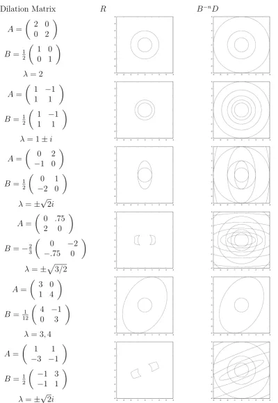
Dilation Matrix R B−n_D

A=

2 0 0 2

B = 1₂

1 0 0 1

λ= 2

A=

1 −1

1 1

B = 1₂

1 −1

1 1

λ= 1±i

A=

0 2

−1 0

B = 1₂

0 1

−2 0

λ =±√2i

A=

0 .75

2 0

B =−2 3

0 −2

−.75 0

λ=±p

3/2

A=

3 0 1 4

B = ₁₂1

4 −1

0 3

λ= 3,4

A=

1 1

−3 −1

B = 1₂

−1 3

−1 1

[image:31.595.78.479.110.690.2]

λ =±√2i

(32)

• there exists some > 0 so that φ is non-zero on the punctured ball {~ω ∈ _Rn _{: 0} _<

k~ωk< }.

Then φ is maximal in ΦA(p).

Proof. Suppose ψ ∈ΦA(p). The first condition tells us exactly that φ(0) = 0⇒ψ(0) = 0.

If φ(~ω) = 0 for some ~ω 6= 0, then we can choose l so φ(~ω) is of the form:

φ(~ω) = p B1~ωp B2~ωp B3~ω. . . p Bl~ωφ Bl~ω,

and Bl_~_ω _{∈ {}_~_ω _∈

Rn : 0 <k~ωk < }. Now as φ Bl~ω 6= 0 we know p Bk~ω = 0 for some

k between 1 andl. But any ψ(~ω) is also of the form:

ψ(~ω) = p B1~ωp B2~ωp B3~ω. . . p Bl~ωψ Bl~ω,

and so will have the same 0 factor in it, and accordingly will be zero.

2.5 Applications in

_R

n

It would be nice to be able to generalise the operator result of Theorem 2.12 from operators onL2₍

R) which commute with D2, to operators on L2(Rn) which commute with DA for a

dilation matrixA. We proved this result for dilation by 2 in_Rby focussing on the solutions of the lattice dilation equation:

f(x) = f(2x) +f(2x−1).

In _R, a lattice dilation equation is one in which the scalea is an integer. This means that it maps any lattice in _R into itself, or a_Z⊂ _Z. In_Rn _{a lattice dilation equation is one in}

which the scale A is a dilation and also AΓ⊂ Γ for some lattice Γ which isn’t flat in _Rn_.

Using a change of basis we can arrange that this lattice is _Zn, and so A must have integer entries [15].

Generalising to other lattice dilations in _R is easy, as for scale a we can just use the lattice dilation equation:

f(x) = f(ax) +f(ax−1) +. . .+f(ax−a+ 1),

when a≥2. If a≤ −2 we use:

f(x) = f(ax+ 1) +f(ax+ 2) +. . .+f(ax−a).

All these equations‡ haveχ[0,1) as a well-behavedL2(R) solution. Armed with these equa-tions and the set of representatives ±[1,|a|), we can proceed through the proof of Theo-rem 2.9 with few changes.

‡_{The second equation is derived from the first using the fact that}_χ

(33)

Theorem 2.20. TheL2(_R) solutions of the above dilation equations are in a natural one-to-one correspondence with the functions in L2₍_±_[1_,_|_a_|₎₎_.

Unfortunately the situation is not so easy to deal with in _Rn_{. Let us consider for a}

moment the important properties which χ[0,1) has. First, it is a maximal solution of a dilation equation. For Theorem 2.9 we use the fact that its Fourier transform stays away from zero on some nice set of representatives, is bounded, and decays reasonably quickly. We then use the fact that it is a generating function for a multiresolution analysis to prove Theorem 2.12. So, given a lattice dilation A on _Rn_{, we want to find a function} _g _which

has all these properties.

2.5.1 Lattice tilings of

_R

n

In _R our well-behaved generating function was the characteristic function for some set. A possible way to generalise this is to look for is for other suitable characteristic functions. One well studied way (see [15]) of doing this is to look for a compact set G with the following properties (up to measure zero):

1. G has distinct translations, ie. G∩(G+~r) =∅ for~r∈_Zn_{\ {}₀_}_.

2. AG the dilated version of Gcan be written as a union of its translations, ie. we can find points~k1, . . . , ~kq so that:

AG=

q

[

i=1

(G+~ki).

3. G covers _Rn _{by translation.}

Rn =

[

~ r∈_Zn

(G+~r).

The first of these conditions tells us that the translates of χG are orthogonal. The second

tells us that χG satisfies a dilation equation and the last tells us that we can get to any

part of _Rn. In fact the~k1, . . . , ~kq turn out to be representatives of the equivalence classes

of A_Zn_/

Zn, of which there are q = |detA|. Remarkably, a set with these properties will even generate a multiresolution analysis.

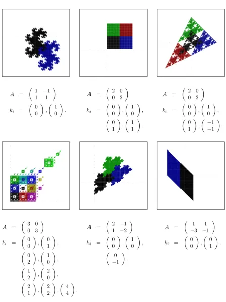
The existence of such sets is even a concrete affair. Any candidate for such a set can be shown to be of the form:

G=

(

~x∈_Rn _:_~_x₌

∞

X

j=1

A−jj, j ∈

n

~k1, . . . , ~kq

o )

.

These summations can be thought of as the base A expansion of points in _Rn _{using the}

(34)

example, if we take A= 2 andk1 = 0, k2 = 1, then we get:

G=

(

x∈_R:x=

∞

X

j=1

j

2j, j = 0 or 1

)

,

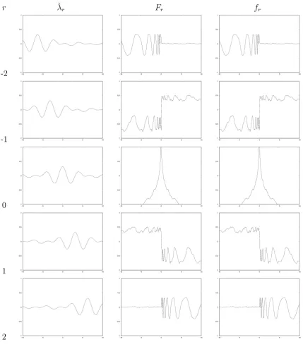
which is the binary expansion of numbers between 0 and 1, so we get [0,1) back again. These candidate sets have the desired properties iff their measure is 1. Figure 2.2 shows various sets G with their dilations A and digit sets. Note that the same A can produce radically different G if different digit sets are chosen.

The next question is: GivenA, when can we select a digit set which will produce aGof measure 1 using the above recipe? In the literature the answer to this question looks rather complicated. To summarise a paragraph of [49], the answer is ‘Always’ in_Rn_for_n _{= 1}_,₂_,₃

and ‘Always’ if |detA| > n; however, the answer is probably ‘Sometimes’ in general. By the time [28] was published a counterexample in _R4 had been found by Potiopa:

A=



  

0 1 0 0

0 0 1 0

0 0 −1 2

−1 0 −1 1



  

.

The reason no suitable digit set can be found for this Arelates to the algebra of rings and to fields generated by roots of its characteristic polynomialx4+x2+ 2.

2.5.2 Wavelet sets and MSF wavelets

The idea of wavelet sets is dual to that of self-similar-affine tilings. This time, instead of producing characteristic functions which generate MRAs, the aim is to produce wavelets whose Fourier transforms are characteristic functions of sets. These wavelets are referred to as minimally supported frequency wavelets, or MSF wavelets. Shannon wavelets, with

ˆ

ψ =χ±[π,2π), are a well-known example of an MSF wavelet in R.

Here existence is not a problem. Dia, Larson and Speegle prove that for any dilation matrixAthere always exists a wavelet set in [6]. They do this by producing a setW which is 2π-translation equivalent to [−π, π)n and B-dilation equivalent to R. This means that

W =S

E~r where:

[−π, π)n= [

~ r∈Zn

E~r+ 2π~r,

and W =S

Fm where:

R = [

m∈Z

BmFm,

(R as given in Theorem 2.18).

The first of these relations tells us that W is much the same shape as [−π, π)n_{and thus}

we can produce L2(W) by using linear combinations of the form:

X

~ r∈Zn

(35)

A =

1 −1 1 1 ki = 0 0 , 1 0 . A = 2 0 0 2 ki = 0 0 , 1 0 , 0 1 , 1 1 . A = 2 0 0 2 ki = 0 0 , 1 0 , 0 1 , −1 −1 . A = 3 0 0 3

ki =

0 0 , 0 1 , 0 2 , 1 0 , 1 2 , 2 0 , 2 1 , 2 2 , 4 4 . A =

2 −1 1 −2

ki =

0 0 , 1 0 , 0 −1 . A = 1 1 −3 −1

ki =

[image:35.595.74.522.90.689.2]

0 0 , 0 1 .

(36)

The second relation tells us that W has the same property as R from Theorem 2.18, that is _Rn₌S

Bm_W_{. This means we can produce}_L2₍

Rn) as a direct sum ofL2(BmW):

X

~r∈_Zn_,m_∈

Z

c~r,me(~r,~ω)χBm_W.

Taking the inverse transform of this equation we findL2₍

R) is the span of:

X

~

r∈Zn,m∈Z

c~r,mw(Am~x−~r),

where w is a constant multiple of the inverse Fourier transform of χW. This makes f a

wavelet for scale A.

The construction of W is presented in a quite abstract form in [6], but [7] contains many nice examples and more of a discussion.

This time, the complication is that we are looking for functions which generate MRAs, not wavelets. Examples of wavelets often arise from an MRA, but these MSF wavelets are primary candidates for counterexamples. Note that there is only a need for one MSF wavelet regardless of the value of det(A), whereas for wavelets arising from an MRA of scale A would require |det(A)| −1 wavelets.

2.5.3 A traditional proof

Having found no suitable maximal solutions to a dilation equation of scaleA, we cannot di-rectly follow the tack we took in_R. However, we can prove a generalisation of Theorem 2.12 using more traditional methods.

Lemma 2.21. Suppose A is a dilation matrix and A is a bounded linear transform on

L2₍

R) which commutes with DA and T~r (for all ~r ∈Zn); then A commutes with all

trans-lations.

Proof. We note that:

TAm_~_r =D_A−mT_~_rD_Am,

so that A commutes with TAm_~_r. Now we show that Am~r is dense in _Rn. Let ~x ∈_Rn and

>0 be given. Note that any point of_Rn _{is within} √n

2 of a point in Z

n_{. Choose}_m_{so that}

kAmk< √2

n, thenA

−m_~_x _{must be within} √n

2 of some~r in Z

n_{. Then:}

k~x−Am~rk ≤ kAmkkA−m~x−~rk

< √2

n

√

n

2 =.

Thus this set is dense in _Rn_{, and so} _A _{commutes with a dense set of translations. By}

the continuity of · 7→ T· and the continuity of A we see that A must commute with all

(37)

Theorem 2.22. Suppose A is a dilation matrix and A is a bounded linear transform on

L2₍

R) which commutes with DA and T~r (for all ~r∈Zn); then A is of the form:

A =F−1πF,

where π∈L∞(_Rn) and π(B~ω) = π(~ω) for all ~ω∈_Rn_.

Proof. By Lemma 2.21A commutes with all translations, and so by Theorem 4.1.1 of [29] (page 92) we can find ρ∈L∞(_Rn) so that:

A=F−1_ρ_F_. That is for any f ∈L2₍

Rn):

F−1ρFf = Af, ρFf = F Af, ρ(~ω) ˆf(ω~) = (F Af) (~ω),

for almost every ~ω∈_Rn_{. Replacing} _f _with _D

Af we get:

ρ(~ω) 1

|detA|fˆ(B~ω) =

1

|detA|(F Af) (B~ω),

ρ(~ω) ˆf(B~ω) = (F Af) (B~ω),

= ρ(B~ω) ˆf(B~ω),

using the last line of the former derivation to replace the RHS. Thus we choose f so that ˆ

f is never zero§ and see that ρ(~ω) =ρ(B~ω) for almost everyω~. We may then adjust ρ on

a set of measure zero to get π.

2.6 Conclusion

We have concocted the idea of a maximal solution m to a transformed dilation equation and shown that such a solution exists for arbitrary p. While this idea of maximality isn’t explicitly stated elsewhere, the idea has certainly been touched upon in the literature (for example Section 8 of [22] or case (c) of Theorem 2.1 in [11]).

There are many possible maximal solutions and we have not invested much time in trying to find m with desirable properties. It is highly likely that by using the properties¶ of p, better behaved m could be found. We have examined the most likely choice for m, the infinite product, and shown that in the usual cases it will be maximal.

We applied this idea of maximality to the Haar dilation equation. Using an idea from [32], that knowing how an operator affects the Haar MRA tells you lots about the operator,

§_{Say, take}_f₍_x_{) =}_e−x2

(38)

we proved some nice results classifying operators which commute with shifts and dilations. It would be interesting to know if our results for an operator A can be extended from ‘A

commutes with D2,T1’ to ‘A sends solutions of scale 2 dilation equations to solutions of the same equation’.

We then generalised these notions to dilation equations on _Rn_{. In our search for a}

suitable MRA to use within the proofs of our operator results we looked at MSF wavelets and self-affine tiles. Both of these families raise many interesting questions. For a given dilation A an MSF wavelet always exists but a self-affine tile may not. It would be inter-esting to investigate a hybrid of these ideas, looking for an MRA generated by a function

g which has ˆg =cχX.

(39)

Chapter 3 Solutions of dilation equations in

L

2

(

_R

)

3.1 Introduction

In Chapter 2 we managed to find the form of all the solutions to a transformed dilation equation, and in particular we nailed down theL2₍

R) solutions tof(x) = f(2x) +f(2x−1) exactly. In this chapter we aim to see if these results are suitable for doing calculations.

3.2 Calculating solutions of

f

(

x

) =

f

(2

x

) +

f

(2

x

−

1)

Using Theorem 2.9 we will actually calculate some solutions tof(x) =f(2x) +f(2x−1). We now know that if g is a solution then:

ˆ

g =πχˆ[0,1),

where π∈L2₍_±_[1_,_{2)) and}_π₍_ω_{) =}_π₍₂_ω_{). Also, for functions ˇ}_ψ _∈_L1₍

R) we know that:

F−1(ψχˆ[0,1)) =cψˇ∗χ[0,1),

where ∗ denotes convolution of two functions and c is a constant depending on the nor-malisation of the Fourier transform. As f(x) = f(2x) +f(2x−1) is linear, we ignore this constant.

As π satisfies π(ω) = π(2ω) it will never∗ be in L2₍

R), so we cannot take its inverse Fourier transform in L2(_R). Likewise it will never satisfy limω→∞|π(ω)| = 0 and so (by

the Riemann-Lebesgue lemma†) cannot be the Fourier transform of an L1₍

R) function. If we are to use the convolution result it will have to be in terms of better-behaved functions.

∗_{Unless trivially}_π_{= 0 almost everywhere.}

(40)

Examining the properties we would expect of ˇπ, we blindly take the inverse Fourier transform of π(ω) =π(2ω) to get:

ˇ

π(x) = 2ˇπ(2x).

It is easy to construct a candidate function for ˇπ. As in the case withπ, it looks like we are free to choose the function on ±[1,2) and then use to the above relation to determine it (almost) everywhere else.

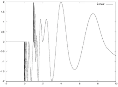
For this example we will take ˇπ(x) to be sin(2πx) on [1,2) and zero on−(2,1]. There are several reasons for this:

• We will be taking the convolution of ˇπ with χ[0,1). Arranging for each “cycle” of ˇπ to have mean zero will simplify this process.

• We will be writing π in terms of sums of:

F sin(2πx)χ[1,2)

.

Using the heuristic “the smoother the function the faster its Fourier transform de-cays” we arrange that sin(2πx)χ[1,2) is continuous to make the convergence of the sums easier to determine‡.

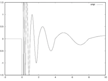
• We leave ˇπ identically zero on_R− as a demonstration of the fact that the two halves are independent.

So we are working with the function:

ˇ

π(x) =

(

2−n_sin(2−n₂_πx₎ _x_∈₂n_[1_,₂₎

0 otherwise ,

a sketch of which is shown in Figure 3.1. We could write this as a sum of sin(2πx)χ[1,2)(x) =

α(x) as follows:

ˇ

π(x) = X

n∈Z

2nsin(2n2πx)χ[1,2)(2nx) =

X

n∈Z

2nα(2nx).

If we cut off this sum above and below we get a sequence of bounded compactly-supported functions. These functions will be in L1(_R) and so we will be able to use the convolution result on these. For m∈_N we define:

ˇ

πm(x) =

|n|<m

X

n∈Z

2nα(2nx)

‡_{Doing the same calculation with cos in place of sin is very slightly harder because cos(2}_πx₎_χ

[1,2)is not

Solutions to dilation equations