Feature Selection in Sparse Matrices

(1)

Feature Selection in Sparse Matrices

Rahul Kumar*_{, Vatsal Srivastava, Manish Pathak}

MIQ Digital, Bangalore, India

Abstract

Feature selection, as a pre-processing step to machine learning, is effective in reducing dimensionality, removing irrelevant data, increasing learning accuracy, and improving result comprehensibility. There are two main approaches for feature selection: wrapper methods, in which the features are selected using the supervised learning algorithm, and filter methods, in which the selection of features is independent of any learning algorithm. However, most of these techniques use feature scoring algorithms that make some basic assumptions about the distribution of the data like normality, balanced distribution of classes, non-sparsity or dense data-set, etc. The data generated in the real world rarely follow such strict criteria. In some cases such as digital advertising, the generated data matrix is actually very sparse and follows no distinct distribution. For this reason, we have come up with a new approach towards feature selection for cases where the data-sets do not follow the above-mentioned assumptions. Our methodology also presents an approach to solve the problem of skewness of data. The efficiency and effectiveness of our methods is then demonstrated by comparison with other well-known techniques of statistics like ANOVA, mutual information, KL divergence, Fisher score, Bayes’ error, Chi-square, etc. The data-set used for validation is a real-world user-browsing history data-set used for ad-campaign targeting. It has very high dimensions and is highly sparse as well. Our approach reduces the number of features to a significant degree without compromising on the accuracy of the final predictions.

Keywords

Feature Selection, Sparse Matrices, Filters Methods

1. Introduction

High-dimensional data, in terms of number of features, is increasingly common these days in different domains. In order to extract useful information from these high volumes of data, one has to use statistical techniques in order to reduce the noise or redundant data. This is because

often we need not use every feature at our disposal for training a model. We can assist our model by feeding in only those features that are really important and are non-correlated. This is where feature selection can play an important role.

The objectives of feature selection at a broad level can be listed as:

(1) To train the model faster

(2) Reduce the complexity of the model and make it easier to interpret

(3) Providing a better understanding of the underlying process that generated the data

(4) To avoid overfitting of our model

In our use case, the data has high dimensions with thousands of features, high class imbalance and sparsity. This project was undertaken in order to reduce the model training time as well as to draw out insights from high performing features and to improve the accuracy of our models.

1.1. Common Filter Methods for Feature Selection and Their Drawbacks

Filter Methodsselect the features on the basis of their scores by various statistical tests for their association with the outcome variable [1]. Different tests are available depending on the nature of the data, the nature of the features and the type of outcome variables i.e. categorical/continuous.

Assumptions generally made by these algorithms are:

 Normality of variables

 Class balance of data-set

 Non-sparsity of data-set

(2)

These assumptions might not be valid for all the real-world datasets. To overcome this problem, we have come up with some new techniques that use some common statistical methods to quantify the separability between the features and make the task of feature selection and dimensionality reduction easier.

2. Data

The dataset that we have is a user-browsing history dataset used for ad-campaign targeting. It has high dimensions and is highly sparse as well. The data is labeled into two classes – converts and non-converts. Converts are the users who fulfill our predefined criteria such as landing at the home-page of a website or making a purchase from the website, etc. and non-converts are the unsuccessful targets who do not satisfy the above-mentioned criteria. The dataset is highly skewed as the number of non-converts constitutes almost 99 percent of the entire dataset.

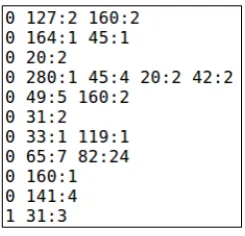
[image:2.595.342.501.78.232.2]

The dataset is stored in a libsvm format. A snapshot of the first 11 rows of the data is shown in Figure 1

Figure 1. First 11 rows of the dataset

2.1. Data Processing

Using the data shown in Figure 1, we create a frequency distribution for each feature. Let us assume that the dataset has N features. So, we will take all the values in feature 0 of the converts dataset and get a frequency distribution of its values. Then we repeat the same process for feature 1, feature 2,... and so on till feature N. At the end of the process we get one directory for each feature in the dataset. Then the same process is repeated for the non_converts dataset. In our example, we will have N different directories which will be named as feature0, feature1, ..., featureN. Inside each directory there will be two files – converts.txt and non_converts.txt. This means we are taking the frequency distribution of values for both the classes separately for each feature.

[image:2.595.391.447.301.411.2]

The file structure after this step is shown in Figure 2

Figure 2. Directory structure after processing the data for frequency distribution

The .txt files will have data in the format given in Figure 3.

Figure 3. An example of the frequency distribution data for a feature

In the above image we can see that the value '0.0' occurs '31327' times, the value '1.0' occurs '427' times, etc.

2.2. Reasons for Sparsity - High Number of Zeroes Most of the datasets are rectangular in shape with thousands of features and billions of rows. Often, the rows represent users and each of the elements of these rows represent the interaction of users with the features.

Now if the number of users and features are large than it is highly probable that a user may not have any interaction with a particular feature. Sometimes, a user may interact with a very small number of features. This potentially results in a highly sparse dataset.

[image:2.595.113.236.360.478.2]

(3)

The sparsity can be seen from the Figure 1 where out of 8903 features in the data-set, the first row has only two with non-zero values (feature127 and feature160 with values 2 and 2 respectively).

2.3. Reasons for Class Imbalance

The meaning of class imbalance is the relatively high difference in the fraction of data points of different labels in the dataset. Class imbalance is quite common in a lot of real-world situations and in different industries. It is certainly a menace in Digital Advertising industry.

There are a variety of reasons for class imbalance. These could be flawed data collection procedure; improper sampling; inherent nature of the dataset and rigorous labeling criteria.

A website can have tremendous traffic. For an ecommerce website, if we only label the users who have made a transaction into positive (converts) class, it will most certainly lead to class imbalance as the ratio of visited users to those making a transaction is extremely high.

Another serious problem posed by class imbalance is the statistical validity of the model. If one of the labels in the dataset is extremely low, the consistency of parameters of the model may be affected. In simple terms, the consistency of a statistical parameter, is the inverse of the amount of deviance in the parameter estimation, as the sample size goes to infinity. This leads to high variance of the model estimated on the skewed data set.

A highly non-separable dataset is also probable due to skewness of the dataset. Many negatively labeled data points may be surrounding the positively labelled data points. Most of the models will not be able to identify the decision boundaries around these positively labelled points. This will lead to model with poor recall value.

3. Statistical Algorithms and Their

Applications to Our Use Case

3.1. Ranking Features Based on the Anova Score and Effect Size

3.1.1. Concept of Anova

Anova [3] is one of the oldest methods to test the causality of a factor (categorical variable) on a continuous variable. The variance of the target variable is partitioned based on factor. The reduction in variance is judged based on a distribution to find out the effect of the factor.

Let y be a factor and x be a continuous variable. In our case, x represents the feature value in the dataset and y

represents the class (converts or non-converts). The variance of x is v with cardinality n. The variable x is partitioned into x1 for converts and x2 for non-converts with cardinality n1 and n2 based on the factor y. The new

variance v1 and v2 are calculated for x1 and x2. The

reduction in variance is expressed as a ratio of new and

initial variance as given by expression (1).

𝑛1𝑣1+𝑛2𝑣2

𝑛𝑣 (1)

This statistic will follow a distribution based on the original distribution of x. The realization of statistic is judged based on distribution to come at the conclusion for the effect of the factor y on x.

3.1.2. Effect Size

Effect size is a simple way of quantifying the difference between the two groups. It has many advantages over using tests of statistical significance alone. Effect size emphasises the size of the difference rather than confounding this with sample size. The effect size is just the standardised mean difference between the two groups, and is expressed as,

𝐸𝑓𝑓𝑒𝑐𝑡𝑆𝑖𝑧𝑒 = 𝜇1−𝜇2

𝑣 (2)

We can use the effect size to rank the features as it is a direct measure of the magnitude of the difference in the two classes. Finding the effect size of each feature and ranking them can give us the knowledge of the importance of each feature.

3.2. Ranking Features Based on Fisher Score 3.2.1. Concept of Fisher Score

Fisher Score [4] is one of the most widely used supervised feature-selection methods. It selects each feature according to their scores under the Fisher criterion.

The key idea of Fisher Score is to find a subset of feature, such that in the data space spanned by the selected feature, the distances between data points in different classes are as large as possible, while the distances between data points in the same class are as small as possible.

We compute a score for each feature independently according to the criterion F. Specifically, let μkj _{and σk}j _be the mean and standard deviation of kth_{class, corresponding} to the jth_{feature. Let μ}j_{and σ}j_{denote the mean and standard} deviation of the whole data set corresponding to the jth feature. Then the Fisher score of the jth_{feature is computed} below,

𝐹(𝑥𝑗_{) =}∑𝑐𝑘=1𝑛𝑘�𝜇𝑘𝑗−𝜇𝑗� 2

�𝜎𝑗_�2 (3) where,

(𝜎𝑗₎2₌_∑𝑐

𝑘=1 𝑛𝑘�𝜎𝑘𝑗� 2

(4) In our case, there are two classes, so c = 2, n is the number of data points in kth_{class and}_j_{represents a} particular feature in the dataset. The value of (σj₎2

calculated for each feature can be used for the purposes of feature ranking.

(4)

and test the effect size that is the difference in the mean divided by variance for each partition. Since our feature has a high number of zeroes, the mean of both partitions tends to zero. This creates the problem of very low effect size.

To overcome this problem, we try reducing the number of zeroes without disturbing the distribution of the overall dataset. We find the proportion of each of the values in the partition is shown in Table 1,

Table 1. Proportion of Values in each partition

Values Percentage

0.0 99.53

1.0 0.02

2.0 0.03

3.0 0.22

4.0 0.15

33.0 0.3

61.0 0.1

75.0 0.1

The data above is skewed towards 0 as it constitutes more than 99 percent of the entire dataset. The mean will therefore, also tend to 0. We try to adjust the concentration of 0's in the data without disturbing the distribution of other values.

Let us take the concentration of each value x to be cx. Now taking new concentration of 0 to be c'0, we define the

modified concentration c'x of each of the other values in the

following manner.

𝑐′𝑥= (1−𝑐0)𝑐𝑥

∑_𝑐𝑥,𝑥≠0𝑐𝑥∀𝑥,𝑥 ≠0 (5) The new set of cx has less concentration of 0's but the

distribution of other values remains the same as their relative concentration is unchanged.

The justification for changing the concentration of c0 is

not difficult. If we look at the way how data has been prepared, the high number of zeroes is because of non-interaction of a user with a feature. In ANOVA and Fisher, we are testing the difference in the mean of the counts converted group and non-converted group. It makes little sense to include those users who have not interacted with a feature at all.

3.4. Ranking the Features Based on Mutual Information

3.4.1. Concept of Mutual Information

Mutual Information [3, 5] is a measure of dependence between two random variables. In probability theory and information theory, the mutual information (MI) of two random variables is a measure of the mutual dependence between the two variables. More specifically, it quantifies the "amount of information" obtained about one random variable, through the other random variable. The concept of

mutual information is intricately linked to that of the entropy of a random variable, a fundamental notion in information theory that defines the "amount of information" held in a random variable.

The Mutual Information between two random variables for feature k is defined as,

𝐼(𝑋𝑘;𝑌) =∑𝑦𝜖𝑌 ∑𝑥∈𝑋𝑘 𝑝(𝑥,𝑦)𝑙𝑜𝑔 �

𝑝(𝑥,𝑦)

𝑝(𝑥)𝑝(𝑦)� (6) In our case, p(Xk, Y) the joint distribution of the feature Xk and Y which is the class label (converts or

non-converts). p(Xk) and p(Y) are the marginal distributions of feature k and class label Y. We can use the value of I(Xk; Y) calculated for each feature for the

purposes of ranking.

3.5. Kullback-Leibler Divergence

3.5.1. Concept of Kullback-Leibler Divergence

The Kullback-Leibler Divergence [3] or KL Divergence measures the difference in two probability distributions. The mathematical formulation is for an individual feature k given as

𝐷𝑘(𝑃||𝑄) =∫_−∞∞ 𝑝(𝑥)𝑙𝑜𝑔𝑝_𝑞(₍𝑥_𝑥)₎𝑑𝑥 (7) where p(x) and q(x) are probability distributions of converts and non-converts for feature k. It can be observed that if p(x) = q(x) for all x, then the measure is 0. In Mutual Information, we are measuring the difference between the joint distribution of two variables, p(X, Y) and the marginal distribution, assuming the two variables are independent. The joint distribution of X and Y will be p(X) * q(Y). In KL Divergence we are calculating the difference between two different distributions p(X) and q(X).

The score Dk(P||Q) calculated for each feature can be

used for the purposes of ranking our features.

3.6. Ranking Features Based on Bayes Error 3.6.1. Classification Using the Discriminant Function

Let X be the feature vector space and K be the set of classes to be classified. To make things simpler, we take two classes C1 and C2 one for converts and the other for

non-converts respectively. The conditional probability density function of feature space for two different classes will be

𝑃(𝑋=𝑥|𝐶=𝐶1) (8) And

𝑃(𝑋=𝑥 | 𝐶=𝐶2) (9) Now to find the discriminant function, we equate the two distributions given by equations 8 and 9. This gives us a function in x, as shown in equation 10,which is the desired discriminant function.

(5)

We classify the regions of the domain to particular class on the basis of their probability. The data-point is assigned to the class with the highest probability among all the classes.

3.6.2. Concept of Bayes' Error

Bayes' error is the cumulative measure of the risk taken while classifying the regions to a particular class. If we classify X = a as class C1 then the risk we are taking is

P(X=a|C=C2). Summing over the domain, we find the total

risk of the classification aka Bayes’ error.

Bayes' error depends upon the decision boundaries. It is imperative that such decision boundaries should have minimum Bayes' Error.

3.6.3. Ranking Features Using Minimum Bayes' Error For each feature, we have the values x1, x2, x3, x4 ... xn.

Taking each value as a discriminant function we form our decision rule:

𝑝𝑟𝑒𝑑𝑖𝑐𝑡𝑒𝑑𝑐𝑙𝑎𝑠𝑠= {0,𝑥<𝑥𝑘 1,𝑥 ≥ 𝑥𝑘 } (11) We find the Bayes’ error using this rule mentioned above and find the minimum error over all xk. The value xk is chosen such that there is a minimum level of wrong classification.

Repeating this for all the features and finding the minimum Bayes’ Error for all of them, we can rank them based on the minimum Bayes' Error.

3.7. Kernel Density Smoothing for Mutual Information, KL Divergence and Bayes’ Error

Kernel Density Smoothing [3] is a non-parametric method to estimate the density of random variable. The method relies on the smoothing the frequency distribution of the random variable. It uses a kernel to extrapolate the distribution at unknown values in the neighbourhood of the point. The following general expression is used for kernel,

𝐾ℎ�𝑋0,𝑋�=𝐷 �‖𝑋−𝑋_ℎ0‖� (12) Where, h is the kernel radius, X, X0are values in the

domain space, D(x) is real-valued decreasing function. For

our purpose we have taken an exponential function for D. Now for a large h we can reduce the influence of abnormal values which in our case is the extremely high frequency of zero values.

3.8. Ranking Features on the Basis of Chi-Square Test Chi-Square [3] Test is used in statistics to test the independence of two events. Chi-Square Score measures how much the expected count E and observed count O deviate from each other. In feature selection, the two events are the occurrence of the feature value and occurrence of a specific class in the dataset. This test is usually applied when both the feature values and the class labels are categorical.

In other words, we want to test whether the occurrence of a specific feature value and the occurrence of a specific class are independent. If the two events are dependent, we can use the occurrence of the feature value to predict the occurrence of the class. We aim to select those features whose values are highly dependent on the occurrence of the class.

When the two events are independent, the observed count is close to the expected count resulting in a small chi-square score (χ2_{). So, a high value of χ}2_{indicates that} the hypothesis of independence is incorrect. In other words, the higher the value of the χ2_{score, the higher the} likelihood that the feature is correlated with the class hence it should be selected for model training.

To apply this test on our dataset, first the continuous data values needed to be converted to categorical values. In order to convert them to categorical value, we take floor of log2 of all the values and aggregate their frequencies. This gives us a dataset of the format shown in Figure 2.

Theoretically, the Chi-Squared parameter for a distribution is given by:

𝜒𝑗2=∑𝑘∈𝐾

�𝑂_𝑗𝑘−𝐸𝑗�2

𝐸𝑗 (13) where O represents the observed frequency and E represents the expected frequency.

Here, in this case, the expected frequency E for jth _feature

is given as

𝐸𝑗=_∑ ∑𝑘∈𝐾(𝑐𝑜𝑛𝑣𝑒𝑟𝑡𝑠𝑎𝑐𝑟𝑜𝑠𝑠𝑎𝑙𝑙𝑏𝑢𝑐𝑘𝑒𝑡𝑠)

𝑘∈𝐾(𝑐𝑜𝑛𝑣𝑒𝑟𝑡𝑠𝑎𝑐𝑟𝑜𝑠𝑠𝑎𝑙𝑙𝑏𝑢𝑐𝑘𝑒𝑡𝑠)+∑𝑘∈𝐾(𝑛𝑜𝑛𝑐𝑜𝑛𝑣𝑒𝑟𝑡𝑠𝑎𝑐𝑟𝑜𝑠𝑠𝑎𝑙𝑙𝑏𝑢𝑐𝑘𝑒𝑡𝑠) (14) where K is the set of buckets after binning. and the observed frequency O for kth_{bucket is taken to be}

𝑂𝑗𝑘 =_{𝑛𝑢𝑚𝑏𝑒𝑟}_𝑜𝑓_{𝑐𝑜𝑛𝑣𝑒𝑟𝑡𝑠}(𝑛𝑢𝑚𝑏𝑒𝑟_𝑖𝑛_{𝑏𝑢𝑐𝑘𝑒𝑡}𝑜𝑓𝑐𝑜𝑛𝑣𝑒𝑟𝑡𝑠_{𝑘+𝑛𝑢𝑚𝑏𝑒𝑟}𝑖𝑛_𝑜𝑓𝑏𝑢𝑐𝑘𝑒𝑡_𝑛𝑜𝑛_{𝑐𝑜𝑛𝑣𝑒𝑟𝑡𝑠}𝑘) _𝑖𝑛_{𝑏𝑢𝑐𝑘𝑒𝑡}_𝑘 (15)

Accordingly, theχ2_{parameter is calculated. The}_{degree of freedom (dof)}_{in this test is (}_{number of buckets-1)}_{. Higher the} χ2_{parameter for a feature more is its importance in model training.}

(6)

4. Results

The dataset we have used for testing has 8903 features. It has the same format as that shown in Figure 1. We randomly sampled twenty percent of the campaign dataset as test data. The testing dataset has around 52.8 million users, out of which around 2600 users are in the positive or converts class.

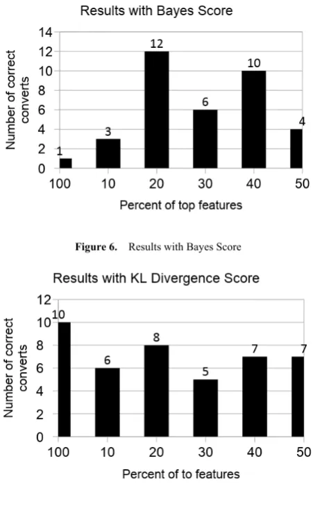
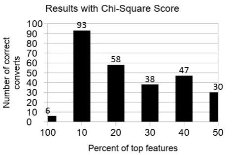
Using the feature ranking techniques as mentioned in Section 3, we give a score to each feature of our dataset. Based on this score, we select the top 10 percent, 20 percent, 30 percent, 40 percent and 50 percent features. Next, we train a Naive Bayes model using only these top n percent features. This model is trained to predict the users who will fall in the converts class. We then compare our results with the model trained without applying any of the above-mentioned feature selection techniques.

[image:6.595.307.533.78.443.2]

We observe that the models trained after applying the feature selection techniques can filter out a significant amount of noise from our dataset. This makes our model more robust and generalized. As can be seen from the figures below, there is a great improvement in the ability of our model to extract the signal from noise when only 10 percent to 20 percent of the highest scored features are taken for each algorithm.

Figure 4. Results with Fisher Score

Figure 5. Results with Mutual Information Score

Figure 6. Results with Bayes Score

Figure 7. Results with KL Divergence Score

[image:6.595.66.282.387.678.2]

(7)

Figure 9. Results with Chi-Square Score

5. Conclusions

Most of the prominent filter methods used for dimensionality reduction makes some basic assumptions about the distribution of the data which might not hold true in the real-world datasets. The approach that we have proposed provides a solution towards feature selection for datasets that are highly sparse in nature with a high class imbalance. The efficiency and effectiveness of our methods can be demonstrated by the fact that we were able to correctly identify almost four times more users of the positive (converted) class using only one-tenth to one-fifth of the total number of features in the dataset. This has not only led to a significant performance boost for our model training pipeline by reducing the size of the training data, but has also made our model more robust and less prone to overfitting as can be seen from the higher number of correct predictions on the test dataset.

REFERENCES

Sánchez-Maroño N., Alonso-Betanzos A., [1]

Tombilla-Sanromán M. (2007). Filter Methods for Feature Selection – A Comparative Study. Intelligent Data Engineering and Automated Learning - IDEAL 2007, 4881, 178-187. DOI: 10.1007/978-3-540-77226-2_19.

Avrim L. Blum and Pat Langley. 1997. Selection of relevant [2]

features and examples in machine learning. Artificial Intelligence 97(1-2), 245-271. DOI: 10.1016/S0004-3702( 97)00063-5.

Guyon, I., Gunn, S., Nikravesh, M., Zadeh, Lotfi A. (2006). [3]

Feature Extraction Foundations and Applications. New York, N Y.: Springer.

Gu, Q., Li, Z., Han, J. (2011). Generalized Fisher Score for [4]

Feature Selection. UAI, 2011b, 266–273.

Doquire, G., Verleysen, M. (2011). A Hybrid Approach to [5]

Feature Selection for Mixed Categorical and Continuous

Data. International Conference on Knowledge Discovery and Information Retrieval, 2011, 394-401. DOI: 10.5220/0003634903940401.

Guyon, I., Elisseeff, A. (2003). An introduction to variable [6]

and feature selection. Journal of Machine Learning Research, 3, 1157-1182.

Yu, L., Liu, H. (2003). Feature selection for [7]

[image:7.595.60.296.77.234.2]