The effectiveness of pole placement method in control system design for an autonomous helicopter model in hovering flight

Full text

(1)International Journal of Integrated Engineering (Issue on Electrical and Electronic Engineering). The Effectiveness of Pole Placement Method in Control System Design for an Autonomous Helicopter Model in Hovering Flight 1. Abas Ab. Wahab1,*, Rosbi Mamat2 and Syariful Syafiq Shamsudin1 Faculty of Mechanical and Manufacturing Engineering, Universiti Tun Hussein Onn Malaysia 2 Faculty of Electrical Engineering, Universiti Teknologi Malaysia *. Corresponding email : [email protected]. Abstract This paper presents the results of attitude, velocity, heave and yaw controller design for an autonomous model scaled helicopter using identified model of vehicle dynamic from parameterized state-space model with quasisteady attitude dynamic approximation (6 Degree of Freedom model). Multivariable state-space control methodology such as pole placement was used to design the linear state-space feedback for the stabilization of helicopter because of its simple controller architecture. The design specification for controller design was selected according to Military Handling Qualities Specification ADS-33C. Results indicate that acceptable controller can be designed using pole placement method with quasi-steady attitude approximation and it has been shown that the controller design was compliance with design criteria of hover requirement in ADS-33C. Keywords: Model Scaled Helicopter, Pole Placement..

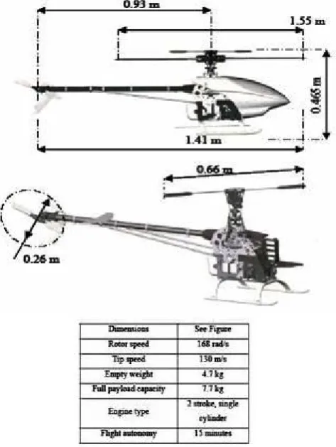
(2) International Journal of Integrated Engineering (Issue on Electrical and Electronic Engineering). 1.. INTRODUCTION. The helicopter was known to be inherently unstable, complicated and nonlinear dynamics under the significant influence of disturbances and parameter perturbations. The system has to be stabilized by using a feedback controller. The stabilizing controller may be designed by the modelbased mathematical approach or by heuristic control algorithms. Due to the complexity of the helicopter dynamics, there have been efforts to apply nonmodel-based approaches such as fuzzy-logic control, neural network control, or a combination of these. Several researchers have proposed PID control (classical control theory) for the autonomous helicopter application such as Amidi (1996), DeBitetto and Sanders (1998) and Montgomey et al. (1993). The classical control approach used by these researchers was used as a low-level vehicle stabilization controller for purpose of attitude, heading and thrust control. The main goal in this research is to provide a working autopilot system for the helicopter model. Therefore, a linear control theory was used because of its consistent performance, well-defined theoretical background and effectiveness proven by many practitioners. In this research, multivariable state-space control theory such as pole placement method has been applied to design the linear state feedback for the stabilization of the helicopter in hover mode. We have chosen the pole placement method because of it simple controller architecture and were suitable for nonlinear system and multiple input multiple output (MIMO) system. Its computational also provided a powerful alternative to classical control theory which eliminated tedious trial and error gain tuning. 2.. Most scaled model helicopters use two bladed rotors and like most of RC helicopter model, Raptor 60 class helicopter uses an unhinged teetering head with harder elastometric restraints, resulting in a stiffer rotor head design. The rotor head designs of scaled model helicopters are relatively more rigid than those in full scaled helicopters, allowing for large rotor control moments and more agile maneuvering capabilities. Since the rotors can exert large thrusts and torques relative to vehicle inertia, Raptor 60 class helicopter rotor head design features stabilizer bar for the ease of handling. Scaled model helicopters are often equipped with mechanical Bell-Hiller stabilizer bar. Invented by Hiller around 1943, the basic principle of operation of the rotor control is to give the main rotor a following rate which compatible with normal pilot responses (Drake, 1980). The following rate is the rate at which the tip path plane of main rotor follows the control stick movements made by the pilot or realigns itself with the mast after an aerodynamics disturbance. According to Mettler et al. (2002), the stabilizer bars receives the same cyclic pitch and roll input from the swash plate but no collective input and has a slower response than main blades. The stabilizer bar is also less sensitive to airspeed and wind gusts due to smaller blade Lock number, γ (ratio between the aerodynamic and internal forces acting on the blade).. AIR VEHICLE DESCRIPTION. The basis of the autonomous UAV Helicopter platform is a conventional remote control (RC) model helicopter, the Raptor 60 class RC Helicopter manufactured by Thunder Tiger Corporation, Taiwan. It has a rotor diameter of 1.605m and is equipped with a high performance Thunder Tiger’s MAX-91SX-HRING C SPEC PS (90 cu in) twostroke petrol engine which produces power about 15kW. The engine is equipped with pump and muffler which pressurized the fuel system to ensure that the engine has stable fuel supply during flight at any altitude and fuel level in tank. Raptor 60 class helicopter has an empty weight about 4.8 kg and capable to carry about 3 kg payloads and an operation time of 15 minutes. General physical characteristics of Raptor 60 class are provided in Fig. 1.. Fig. 1 Raptor 60 class RC helicopter physical characteristics.

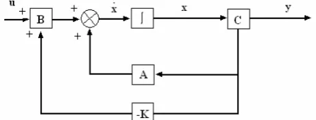
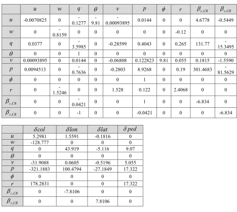
(3) International Journal of Integrated Engineering (Issue on Electrical and Electronic Engineering). 3.0 DYNAMICS OF SCALED MODEL RAPTOR 60 CLASS HELICOPTER Helicopter dynamics obey the Newton-Euler equation for rigid body in translational and rotational motion. The helicopter dynamic can be studied by employing lumped parameter approach which indicates that helicopter as the composition of following component; main rotor, tail rotor, fuselage, horizontal bar and vertical bar. The parameterized state-space model can be described with the following state (refer Fig. 2 for coordinate axis) and control input vector consisting 4 components of lateral cyclic, longitudinal cyclic, tail rotor collective and main rotor collective (Mettler et al., 2000), (Heffley and Mnich, 1986). x = {u , w, q, θ , v, p, φ , r , β c ,CR , β s ,CR }. (1). u = [δ lat δ lon δ ped δ col ]. (2). where u, v, w are the velocities in the fuselage coordinates, p, q, r are the roll, pitch and yaw angular rate, φ , θ are the roll and pitch attitude angles about the principal fuselage axis, β c ,CR , , β s ,CR (c, d) represent the longitudinal and lateral stabilizer bar flapping angles for a first order tip path plane model. The system and control matrices F and G for hover are listed in Appendix A show all of the important gravitational terms that can be obtained analytically and partial derivatives arising from aerodynamic forces and moments necessary to describe the linear set of equations for a helicopter. The linear, first-order set of differential equations is given in the form of Equation 3 and the detailed derivation of partial derivatives is given in Padfield (1996) and Prouty (1986). .. x = F x + Gδ u. (3). The system matrix F includes derivatives due to small perturbations of system states; the control matrix G represents the derivatives due to small perturbations of control inputs. The stability derivative for parameterized state-space matrices is listed in Table 1 (Appendix B). The model has simple block structure and the dynamic of model scaled helicopter can be sufficiently decoupled to allow an analysis of lateral/longitudinal dynamics separately from. yaw/heave dynamics in hover condition. The standard rotorcraft handling qualities matrices outline by US Army Aviation Systems Command (1989) can be used to analysis rotorcraft dynamic.. Fig. 2 Helicopter variables with fuselage coordinate system and rotor/stabilizer bar states (Mettler et al., 2000).. 4.0 STATE DESIGN. SPACE. CONTROLLER. A typical feedback control system in Fig. 3 can be represented in state space system as Equation 4 and 5 where the light lines are scalars and the heavy line are vectors. .. x = A x + Bu y =C x. (4) (5). Fig. 3 A typical state space representation of a plant.. In the typical feedback control system, the output ( y ) is fed back to the summing junction. In linear state feedback design, each state variable is fed back to the control, u , through a gain, k i to yield the required closed-loop pole values. The feedback through the gains k i is represented in Fig. 4 by the feedback vector –K..

(4) International Journal of Integrated Engineering (Issue on Electrical and Electronic Engineering). attitude controller design, the percentage of overshoot (OS) is set to be 10% and the settling time of 5 second should be achieved with no steady state error.. Fig. 4 A state space representation of a plant (Nise, 2000).. The state equation for close loop system of Fig. 4 can be written by inspection as. x& = Ax + Bu = Ax + B( −Kx + r ) = ( A − BK ) x + Br (6) (7) y = Cx The design of state variable feedback for closed loop pole placement consists of equating the characteristic equation of a closed loop system to a desired characteristic equation and then finding the values of feedback gains, k i . The gain, k i value can be solved using MATLAB® using function ‘acker’ for SISO system and ‘place’ for MIMO system.. 5.0. RESULTS AND DISCUSSION. Equation (1) can be analyzed separately in longitudinal and lateral stability augmentation, heave and yaw dynamic mode. All state variables in the Equation (1) were also assumed to be measurable while designing controller using pole placement method.. 5.1. Attitude Controller Design. The attitude dynamics indicates the behavior when the translational motion in x and y is constrained. For the design of attitude feedback design, the dynamic model was extracted by fixing the state variables of translational velocities in x, y and z direction and the yaw terms to zero. The design specification for the controller design is selected according to Aeronautical Design Standard for military helicopter (ADS33C), (US Army Aviation Systems Command, 1989). In Fig. 5, the damping ratio limits on pitch (roll) oscillations in hover and low speed is specified to be greater than 0.35 (OS% ≤ 30.9) and the settling time to be achieved less than 10 second. Therefore for the purpose of. Fig. 5 Limits on pitch (roll) oscillations – hover and low speed according to Aeronautical Design Standard for military helicopter (ADS-33C) (US Army Aviation Systems Command, 1989).. Using the ‘place’ and ‘ltiview’ function in MATLAB®, the performance of attitude controller can be achieved according to design requirement for the both pitch and roll axis. In the pitch axis response, the poles are placed at p = -0.8 + 1.095i, -0.8 – 1.095i and -0.00842 in order to achieve 10% OS and 5 second settling time and the phase variable feedback gain is found to be K θ = [0 − 0.4527 0.0136] . In the roll axis response, the poles are placed at p = 0.8 + 1.095i, -0.8 – 1.095i and -0.5219 in order to achieve 10% OS and 5 second settling time and the phase variable feedback is found to be K φ = [− 0.0015 − 0.5508 0.0084] . The time response and bode diagram plot for both axes are shown in Fig. 6(a) and Fig. 6(b). In Fig. 7, both controller bandwidth and time delay have been shown to meet Level 1 requirement specify in Section 3.3.21 of the Military Handling Qualities Specification ADS-33C..

(5) International Journal of Integrated Engineering (Issue on Electrical and Electronic Engineering) -3. Linear Simulation Results. x 10. 8 7. A m p litu d e P itc h A n gle (ra d ). 6 5 4 3 2 1 0. 0. 1. 2. 3. 4. 5 Time (sec). 6. 7. 8. 9. 10. Bode Diagram. M a g nitu de ( dB ). 20 0. -20 -40 -60. P h as e (d e g). -80 0 -45 -90. -135 -180 -3 10. -2. -1. 10. 0. 10. 1. 10. 2. 10. Fig. 7 Compliance with small-amplitude pitch (roll) attitude changes in hover and low speed requirement specified in Section 3.3.2.1 of the Military Handling Qualities Specification ADS-33C.. 10. Frequency (rad/sec). Fig. 6(a) Attitude compensator design for pitch axis response due to 0.007 rad longitudinal cyclic step command. The phase variable feedback gain is found to be Kθ =[0.009 −0.0455 0.0417] . The bandwidth, ω BWθ is located at 2.39 rad/s and the phase delay,. 5.2. τ Pθ = 0.. Linear Simulation Results 0.035 0.03. A m p litu d e R o ll A ng le ( ra d ). 0.025 0.02. 0.015 0.01 0.005 0. 0. 1. 2. 3. 4. 5 Time (sec). 6. 7. 8. 9. 10. Bode Diagram. M a gn itud e ( d B). 20 0. -20 -40 -60. P h as e ( d eg ). -80 0 -45 -90. -135 -180 -2 10. -1. 10. 0. 10 Frequency (rad/sec). 1. 2. 10. 10. Fig. 6(b) Attitude compensator design for roll axis response due to 0.0291 rad lateral cyclic step command. The phase variable feedback gain is found to be Kφ =[ 0.0103 −0.3872 −0.0673] . The bandwidth, ω BWφ is located at 2.37 rad/s and the phase delay,. τ Pφ = 0.. Velocity Control. Once the attitude dynamics are stabilized, the feedback gain for the velocity dynamic can be determined with similar approach. For velocity control, the design of the phase variable feedback gains should yield 10% overshoot and a settling time of 5 second. In longitudinal velocity mode, the poles was selected to be placed at p = -0.8 + 1.095i, -0.8 – 1.095i and 57.7 in order to achieve 10% OS and 5 second settling time and the suitable feedback gains were found to be K u = [ −0.2428 1.2783 2.1660] for longitudinal velocity. In lateral velocity mode, the poles was selected to be placed at p = -0.8 + 1.095i, -0.8 – 1.095i and -5 in order to achieve 10% OS and 5 second settling time and the suitable feedback gains were found to be K v = [ −0.028 −0.5682 −0.3481] for lateral velocity. Fig. 8(a) and 8(b) shows the step response of the velocity dynamic in longitudinal and lateral modes..

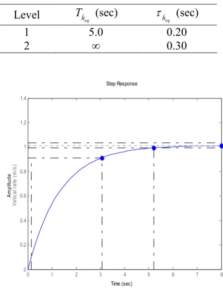
(6) International Journal of Integrated Engineering (Issue on Electrical and Electronic Engineering) Step Response 1.4. 1.2. Amplitude horizontal velocity, u (m/s). 1. 0.8. 0.6. 0.4. 0.2. 0. 0. 2. 4. 6. 8. 10. 12. Time (sec). Fig. 9 Procedure for obtaining equivalent time domain parameters for height response to collective controller according to Aeronautical Design Standard for military helicopter (ADS-33C) (US Army Aviation Systems Command, 1989).. Fig. 8(a) Velocity compensator design for longitudinal velocity mode due to longitudinal cyclic step command. Table 2 Maximum values for height response parametershover and low speed according to Aeronautical Design Standard for military helicopter (ADS-33C) (US Army Aviation Systems Command, 1989).. Step Response 1.4. 1.2. Level 1 2. Am p litud e L ate ral Veloc ity , v (m /s ). 1. 0.8. Th&eq (sec). τ h& (sec). 5.0 ∞. 0.20 0.30. eq. 0.6. Step Response 0.4. 1.4. 0.2. 1.2. 0. 1 0. 1. 2. 3. 4. 5. 6. Fig. 8(b) Velocity compensator design for lateral velocity mode due to lateral cyclic step command.. 5.3. Heave and Yaw Control. The heave dynamics were represented as a first order system transfer function and further damping by velocity feedback improves the system response considerably. ADS-33C has listed a procedure for obtaining the equivalent time domain parameters for the height response to collective controller in Fig. 9. For Level 1 handling quality define in Cooper-Harper Handling Qualities Rating (HQR) Scale, the vertical rate response shall have a qualitative first order appearance for at least 5 second following a step collective input (See Table 2). In order to achieve this, the gains are chosen to be K w = -2.14. The step response for the heave controller is shown in Fig. 10.. Am plitude Vetic al rate (m /s ). Time (sec). 0.8. 0.6. 0.4. 0.2. 0. 0. 1. 2. 3. 4. 5. 6. 7. 8. Time (sec). Fig. 10 Heave dynamics compensator design due to collective pitch step command.. The yaw controller can be design in similar way to heave controller. For yaw response to lateral controller, the design of the phase variable feedback gains should bandwidth and time delay specified in Section 3.3.21 of the Military Handling Qualities Specification ADS33C. The poles were placed at p = -0.2 and -3 in.

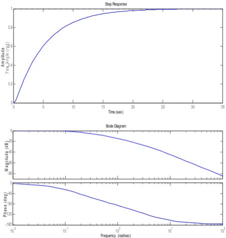
(7) International Journal of Integrated Engineering (Issue on Electrical and Electronic Engineering). order to achieve the design requirement. Based on the step and bode diagram response of the velocity dynamic shown in Fig. 11, the suitable feedback gains were found to be Kψ = [ 0.3237 0.0346] . In Fig. 12, yaw controller bandwidth and time delay have been shown to meet Level 1 requirement specify in Section 3.3.21 of the Military Handling Qualities Specification ADS-33C. Step Response 1. A m p litu d e Y a w A n g le ( r a d ). 0.8. 0.6. 0.4. 0.2. 0. 0. 5. 10. 15. 20. 25. 30. 35. Time (sec) Bode Diagram 0 M a g n itu d e ( d B ). -20 -40 -60 -80 0. P has e (deg). -45 -90. -135 -180 -2 10. 10. -1. 0. 10 Frequency (rad/sec). 10. 1. 2. 10. Fig. 11 Yaw dynamics compensator design due to tail rotor collective pitch step command. The phase variable feedback gain is found to be Kψ = [ 0.3237 0.0346 ] . The bandwidth,. ω BWφ. is located at 3.42 rad/s and the phase delay,. τ Pφ = 0.. Fig. 12 Compliance with small-amplitude heading changes in hover and low speed requirement specified in Section 3.3.5.1 of the Military Handling Qualities Specification ADS-33C.. 6.0. SYSTEM EVALUATION – FLIGHT TEST. The flight test for evaluation of control law design had been conducted in three phases where the helicopter model was tested to perform hover maneuver (Syariful Syafiq Shamsudin, 2007). The complete autopilot design and system integration works have been discussed briefly in Syariful Syafiq Shamsudin et al. (2006). The third phase of the flight test is designed to stabilize the helicopter flight using partially computer control. During this phase, three of the receiver output channels were controlled under computer guidance whiles all others manually. Partial computer controlled flight was when the pilot flew only one channel of control (Collective pitch/Throttle) and the computer flew the remaining channels (Fig. 13). Most of the flight testing of the aircraft had been done in this mode. The purpose of this flight testing was to allow for the tuning of the flight control system, one channel at a time. The computer flew the longitudinal cyclic, lateral cyclic and yaw channel. Once each channel had been tuned up separately, the combinations were then turned over to computer control. This type of flight testing was done on a regular basis. During these testing, telemetry data was being used to monitor the performance of the avionics while in flight. At no point during these testing did any of the electronics fail while the aircraft was flying. The experiment results of the hovering controller tested on the Raptor .90 helicopter model are shown in Fig. 6.19, 6.20 and 6.21 for roll, pitch and yaw angle stabilization respectively. The UAV showed a stable attitude response over two minutes and began to sway slowly from the current hovering position since the positional controller is not implemented. The graph shows that the roll angle is regulated within ± 2°~3° (± 0.3049~0.0524 rad), pitch angle is within ± 3°~4° (± 0.0524~0.0698 rad) and yaw angle is within ± 99°~103° (± 1.7279~1.7977 rad)..

(8) International Journal of Integrated Engineering (Issue on Electrical and Electronic Engineering). Fig. 13 Partially computer control flight test. Fig. 16 Experiment results of attitude (yaw angle) regulation by autopilot system. 7.0. Fig. 14 Experiment results of attitude (rollangle) regulation by autopilot system. Fig. 15 Experiment results of attitude (pitch angle) regulation by autopilot system. CONCLUSION. The paper has shown results of using state feedback method in designing attitude, velocity, heave and yaw controller for the autonomous helicopter model. Parameterized state space model was reduced to rigid body form with quasi-steady attitude approximation and can be decoupled to allow an analysis of lateral/longitudinal dynamics separately from yaw/heave dynamics in hover condition. The phase variable feedback gains were calculated for each helicopter dynamics in hover condition to satisfy the requirements contained in the ADS-33C. The performance of autopilot system developed had been evaluated through the tests conducted in test rig, preliminary test and actual flight test. The proposed hovering controller has shown capable of stabilizing the helicopter attitude angles. The positional, velocity and heave controller design could not be implemented in the tests due to limitation of resources in this project. A GPS device should be used as part of autopilot’s sensor to give position information to flight computer. The combination of AHRS and GPS device could enable better hovering stabilization control of helicopter model with position hold capabilities..

(9) International Journal of Integrated Engineering (Issue on Electrical and Electronic Engineering). 8.0. ACKNOWLEDGEMENTS. The funding for this research was supported by UTM Fundamental Research Grant Vot 75124 and UTM-PTP scholarship.. 9.0. NOMENCLATURES. β c ,CR , , β s ,CR (c, d). ki p, q, r u, v, w Xu, Yv, Lu, Lv, Mu. φ, θ. 10.0. The longitudinal and lateral stabilizer bar flapping angles for a first order tip path plane model Required closed-loop pole values The roll, pitch and yaw angular rate The velocities in the fuselage coordinates General aerodynamic effects expressed by speed derivatives The roll and pitch attitude angles about the principal fuselage axis. REFERENCES. [1] Amidi, O. (1996), An Autonomous Vision Guided Helicopter, PhD Thesis, Carnegie Mellon Universities, Pittsburgh. [2] US Army Aviation Systems Command (1989), Handling Qualities Requirements for Military Rotorcraft, US Army AVSCOM Aeronautical Design Standard, ADS-33C. [3] DeBitetto, P.A and Sanders, C.P (1998), Hierarchical Control of Small Autonomous Helicopters, Proceeding of The 37th IEEE Conference on Decision and Control, Florida, USA. [4] Drake, John A. (1980), Radio Control Helicopter Models, Watford, Herts: Model and Allied. [5] Heffley, Robert K. and Mnich, Marc A. (1986), Minimum Complexity Helicopter Simulation Math Model Program, Manudyne Report 83-2-3, NASA Ames. Research Center, NAS2-11665, Moffet Field, CA 94035. [6] Mettler, B., Tishler, M.B and Kanade, T. (2000), System Identification Modeling of a Model-Scale Helicopter, Technical Report CMU-RI-TR-00-03, Robotics Institute, Carnegie Mellon University. [7] Mettler, B., Dever, C. and Feron, E. (2002), Identification Modeling, Flying Qualities and Dynamic Scaling of Miniature Rotorcraft, NATO Systems Concepts & Integration Symposium, Berlin. [8] Montgomery, J.F, Fagg, A.H, Lewis, M.A, Bekey, G.A (1993), The USC Autonomous Flying Vehicles: An Experimental in Real Time Behavior Based Control, Proceeding of the 1993 IEEE/RSJ International Conference on Intelligent Robots and Systems. [9] Nise, Norman S. (2000), Control System Engineering, John Wiley & Sons Inc., New York [10] Padfield, G.D (1996), Helicopter Flight Dynamics: The Theory and Application of Flying Qualities and Simulation Modeling, AIAA Education Series, Reston, VA. Prouty, R.W (1986), Helicopter [11] Performance, Stability and Control, PWS Engineering, Boston. Syariful Syafiq Shamsudin, Abas [12] Ab. Wahab and Rosbi Mamat (2006). The Development of Autopilot System for UTM Autonomous UAV Helicopter Model 1st Regional Conference on Vehicle Engineering and Technology (RIVET 2006). 3-5 July, Kuala Lumpur: Automotive, Aeronautic & Marine Focus Group, RMC, UTM. [13] Syariful Syafiq Shamsudin (2007). The Development of Autopilot System for Unmanned Aerial Vehicle (UAV) Helicopter Model. M.Eng Thesis, Universiti Teknologi Malaysia..

(10) International Journal of Integrated Engineering (Issue on Electrical and Electronic Engineering). APPENDIX A. System and Control Matrices. δ col , MR = θ 0 Commanded main rotor collective angle δ long = B1, SP Longitudinal swashplate tilt δ lat = A1, SP Lateral swashplate tilt δ col ,TR = θOT Commanded tail rotor collective angle.

(11) International Journal of Integrated Engineering (Issue on Electrical and Electronic Engineering). APPENDIX B Table 1 Analytically obtained system matrix in hover. u. w. q. θ. v. p. φ. r. β c ,CR. β s ,CR. u. -0.0070825. 0. 0.1277. 9.81. 0.00093895. 0.0144. 0. 0. 4.6778. -0.5449. w. 0. 0.8159. 0. 0. 0. 0. 0. -0.12. 0. 0. q. 0.0377. 0. 0. -0.28599. 0.4043. 0. 0.265. 131.77. θ v. 0 0.00093895. 0 0. 0 0. 0 -0.06808. 0 0.122823. 0 9.81. 0 0.055. 0 0.1815. p. 0.0094513. 0. 0. -0.2803. 8.9268. 0. 0.19. 301.4683. φ. 0. 0. 0. 1. 0. 0. 0. r. 0. 0 1.5246. 15.3495 0 -1.5590 81.5629 0. 0. 0. 1.528. 0.122. 0. 2.4068. 0. 0. β c ,CR. 0. 0. 0.0421. 0. 0. 1. 0. 0. -6.834. 0. β s ,CR. 0. 0. -1. 0. 0. -0.0421. 0. 0. 0. -6.834. 3.5985 1 0.0144 0.7636 0. δ col. δ lon. δ lat. δ ped. r. 5.2981 -128.777 0 0 -31.9088 -321.1883 0 178.2831. 1.5591 0 43.919 0 0.0605 100.4794 0 0. -0.1816 0 -5.116 0 -0.5196 -27.1849 0 0. 0 0 9.07 0 5.055 17.322 0 17.322. β c ,CR. 0. -7.8106. 0. 0. β s ,CR. 0. 0. 7.8106. 0. u w q. θ v p. φ.

(12)

No results found