THE THROUGHPUT FOR MULTI HOP RELAY WIRELESS SENSOR NETWORKS BASED ON COOPERATIVE DIVERSITY

(1)

ISSN: 1992-8645 www.jatit.org E-ISSN: 1817-3195

SYNCHRONIZATION OF A CLASS OF COMPLEX

NETWORKS WITH NETWORKED COUPLING CHANNELS

1_{WEIKE SHANG,} 2_{XINXIN FU,}3_{JIN ZHU,} 4_{HONGSHENG XI}

All the authors are with Department of Auto, University of Science and Technology of China, Hefei, 230027, Anhui, China

ABSTRACT

The synchronization problem is investigated for a class of discrete-time complex networks, where the networking induced communication constraints between the coupling nodes are considered. By choosing a novel Lyapunov functional, sufficient conditions for the synchronization of the discrete-time complex networks subject to both coupling delays and packet dropouts are given. The derived criteria are presented in the form of linear matrix inequalities (LMIs), which is easy to be solved numerically. Finally, an illustrative example is presented to verify the effectiveness of the results.

Keywords:Global synchronization, stochastic complex networks, coupling delays, packet dropouts

1. INTRODUCTION

Complex networks have received considerable attention over the past decades. They are ideal mathematical models for various natural and engineering systems: cellular networks, social systems, the Internet, just to name a few [1]~[16]. The scientific interests in complex networks include, for example, the clustering characteristic (small world effect) and degree distributions, [1]~[3]; the stability and synchronization of complex networks, [4]~[16] and so on.

Due to the finite speeds of transmission and spreading, traffic congestions, as well as bandwidth restriction(for the Internet), information travelling through a complex network is often associated with time delay as well as packet dropouts. This is ubiquitous in biological, physical and engineering networks. Time-delay often causes instability of the system and thus has been investigated extensively in various contexts for complex networks: for deterministic systems the reader is referred to [7], [14]; for stochastic modeling and analysis please refer to [17]~[19]; besides, [20], [21] provide good hints for nonlinear systems. Packet dropouts have also received much attention in recent years, as they are inevitable in imperfect communication networks [22]~[25]. They are firstly treated separately from time-delays, but more recent models intend to combine the two effects together, which is more practical. In most studies, the packet dropout process is modeled as a Bernoulli process with

appropriate variations in correspondence to the specific systems.

To the best of the authors’ knowledge, the synchronization problem for complex networks subject to the communication constraints is still an open problem, which motivates the present work. The main contributions of the paper are threefold: (1) the imperfect coupling communication channels are considered for the first time in the synchronization context. (2) a stochastic model is utilized to describe the incomplete information phenomenon, taking both coupling delays and data packets dropout into account, and covering the aforementioned models as its special cases. (3) the stochastic analysis methods, the properties of Kronecker product, as well as the free-weight matrix techniques are employed to deal with the synchronization problem, and criterions in terms of linear matrix inequalities (LMIs) are given.

The rest of this paper is organized as follows. In Section 2, the discrete-time complex networks with coupling communication constraints induced by the imperfect networked channels is introduced, and then the problem under consideration is formulated. In Section 3, sufficient conditions are presented to guarantee the synchronization for the considered complex networks. An illustrative example is given in Section 4 to demonstrate the feasibility of the acquired criterion. Finally, concise conclusions are drawn in Section 5.

(2)

the set of all 𝑚×𝑛 real matrices. The superscript ‘T’ denotes matrix transposition and ‘*’ denotes the transpose of corresponding elements introduced by symmetry. 𝑋> 0 means that 𝑋 is real symmetric and positive definite; Moreover, 𝑋>𝑌 means

𝑋 − 𝑌> 0. 𝐼 and 0 represent the identity matrix and zero matrix with compatible dimensions, respectively. Given a matrix 𝐴, denote by ∥ 𝐴 ∥ its operator norm, i.e.∥ 𝐴 ∥=𝑠𝑢𝑝{|𝐴𝑥|∶|𝑥| = 1} =

�𝜆𝑚𝑎𝑥(𝐴𝑇𝐴), with | | denoting the Euclidean norm on ℝn, and ¸ 𝜆_𝑚𝑎𝑥(𝑄) denoting the maximal eigenvalue of square matrix 𝑄. (𝛺,ℱ, {ℱ_𝑘}_𝑘∈𝑁)is a complete probability space with a filtration {ℱ_𝑘} satisfying the usual conditions (i.e. ℱ_𝑘 contains all the 𝑃 −null sets and it is right continuous). 𝔼{∙} is the mathematical expectation of a random variable with respect to the given probability space, and

𝔼{𝜉|𝜒} denotes the conditional mathematical

expectation of a random variable 𝜉 ∈ ℱ with respect to the subfield created by 𝜒 (i.e. 𝜎(𝜒)). All the matrices, if they are not explicitly specified, are assumed to have compatible dimensions.

2. PROBLEM FORMULATION AND

PRELIMINARIES

The following discrete-time complex network with nonlinearity and multiple time-delays is considered

𝑥𝑚(𝑘+ 1) =𝐴𝑥𝑚(𝑘) +𝐵𝑓�𝑥𝑚(𝑘)�

+𝐵𝑑𝑔 �𝑥𝑚�𝑘 − 𝑑(𝑘)��

+� � 𝜔𝑚𝛼(𝑝)𝐼𝑝(𝑘)Γ𝑝𝑥𝛼(𝑘 𝑟

𝑝=0 𝑁

𝛼=1

− 𝜏𝑝(𝑘)) 𝑚= 1,2,⋯,𝑁

(1)

where𝑥_𝑚(𝑘),𝑥_𝑚�𝑘 − 𝑑(𝑘)�, 𝑥_𝛼(𝑘 − 𝜏_𝑝(𝑘)∈ ℝ𝑛 denote the state vector, delayed state vector, and the coupling delayed vector of the mth node of the complex networks at time k respectively. 𝐴,𝐵,𝐵_𝑑 are all known matrices with compatible dimensions.

𝑓,𝑔:ℝ𝑛_{→ ℝ}𝑛_{are both vector-valued nonlinear}

functions to be given later. 𝑑(𝑘), 𝜏𝑝(𝑘) are

integers denoting the state time-delay and all the possible coupling delays which satisfy:

𝑑 ≤ 𝑑(𝑘)≤ 𝑑 (2)

𝜏0(𝑘) = 0 (3)

𝜏𝑝≤ 𝜏𝑝(𝑘)≤ 𝜏𝑝 𝑝= 1,2,⋯,𝑟 (4)

where 𝑑, 𝑑, 𝜏_𝑝and 𝜏_𝑝(𝑝= 1,2,⋯,𝑟) are all known

positive integers. Moreover we define that 𝑑_𝑚𝑎𝑥=

max𝑝( 𝜏𝑝,𝑑). 𝛤𝑝 denotes the inner-coupling matrices linking the

𝛼

th coupling state variable

with time-delay 𝜏_𝑝(𝑘), 𝑊(𝑝) = (𝜔_𝑚𝛼(𝑝))_𝑁_×_𝑁 is the outer-coupling configuration matrix of the network with 𝜔_𝑚𝛼_,_𝑝≥0(𝑚 ≠ 𝛼), but not all zeros, and the coupling configuration matrix 𝑊(𝑝)(𝑝= 0,1,⋯,𝑟) is assumed to satisfy the diffusive connections:

𝜔𝑚𝛼(𝑝) =𝜔𝛼𝑚(𝑝) ,𝑚 ≠ 𝛼

� 𝜔𝑚𝛼(𝑝) 𝑁

𝑚=1

=� 𝜔𝑚𝛼(𝑝)

𝑁

𝛼=1

= 0 ,

𝑚,𝛼= 1,2,⋯,𝑁; 𝑝= 0,1,⋯,𝑟

𝐼𝑝(𝑘) is assumed to be a random variable satisfying certain discrete probabilistic distributions on the

interval [0,1] which can be acquired from statistical tests, mutually unrelated with each other (for

𝑝= 0,1,⋯,𝑟) with mathematical expectation𝛼_𝑝

and variance𝛾_𝑝2.

Assumption 2.1: The nonlinear function

𝑓(𝑥(𝑘)),𝑔(𝑥(𝑘)):ℝ𝑛_{→ ℝ}𝑛 _{are assumed to be}

satisfying the following sector nonlinearity described as

[𝑓(𝑥)− 𝑓(𝑦)− 𝐾1(𝑥 − 𝑦)]𝑇[𝑓(𝑥)− 𝑓(𝑦)

− 𝐾2(𝑥 − 𝑦)]≤0 ,∀𝑥,𝑦 ∈ ℝn

(5)

[𝑔(𝑥)− 𝑔(𝑦)− 𝐿1(𝑥 − 𝑦)]𝑇[𝑔(𝑥)− 𝑔(𝑦)

− 𝐿2(𝑥 − 𝑦)]≤0 ,∀𝑥,𝑦 ∈ ℝn

(6)

both of which satisfy the zero initial condition, i.e.

𝑓(0) = 0,𝑔(0) = 0, and 𝐾₁,𝐾₂,𝐿₁,𝐿₂ are all known matrices satisfying 𝐾₁− 𝐾₂< 0,𝐿₁− 𝐿₂<

0.

Remark 2.1: The model in(1) includes both delayed (for 𝑝= 1,2,⋯,𝑟 ) and non-delayed coupling (for 𝑝= 0,), which makes it very general, and can cover most of the existing models.

(3)

sequence of random variables with arbitrary discrete probabilistic distributions in this paper defined on [0 1] in this paper to be Bernoulli distributions. The assumption in this paper is reasonable because in practice the transmitted information can be neither completely missing nor completely received, but only a part of the initial information can be transmitted successfully. In that case, the usually assumed Bernoulli distribution which only takes the completely successful case and the completely missing case in account is not quite suitable. Similar ideas can be referred to [26], [27], and [28], which focuses on the missing measurements without taking multiple time-delays into account.

Firstly, for simplicity denote

𝑥(𝑘) =𝑐𝑜𝑙{𝑥1(𝑘),𝑥2(𝑘),⋯,𝑥𝑁(𝑘)}

𝑓(𝑥(𝑘)) =𝑐𝑜𝑙{𝑓(𝑥₁(𝑘)),𝑓(𝑥2(𝑘)),⋯,𝑓(𝑥𝑁(𝑘))}

𝑔(𝑥(𝑘)) =𝑐𝑜𝑙{𝑔(𝑥1(𝑘)),𝑔(𝑥2(𝑘)),⋯,𝑔(𝑥𝑁(𝑘))}

𝛼𝑝=𝐸�𝐼𝑝(𝑘)� , 𝛾𝑝2= E��𝐼𝑝(𝑘)− 𝛼𝑝�2�

Γ𝑝=𝛼𝑝×Γ𝑝 𝑝= 0,1,⋯ 𝑟

𝑊(𝑝)_{= (𝜔}

𝛼(𝑝))𝑁×𝑁

𝑊(𝑝)_𝑊(𝑞) ₌_𝑊(𝑝,𝑞)_{= (𝜔}

𝑚𝛼(𝑝,𝑞))𝑁×𝑁 𝑝,𝑞= 0,1,⋯ 𝑟 By the Kronecker product ‘⨂’ of matrix, the complex networks dynamics of (1) can be recast into the following compact form

𝑥(𝑘+ 1) = (𝐼⨂𝐴+ I0(𝑘) ×𝑊0⨂Γ0)𝑥(𝑘)

+ (𝐼⨂𝐵)𝑓(𝑥(𝑘))

+ (𝐼⨂𝐵𝑑)𝑔 �𝑥�𝑘 − 𝑑(𝑘)��

+�I𝑝(𝑘) ×�𝑊(𝑝)⨂Γ𝑝�𝑥(𝑘

𝑟

𝑝=1

− 𝜏𝑝(𝑘))

(7)

Moreover, to make the deduction more concise, the augmented complex networks can be denoted in the following form

𝑥(𝑘+ 1) =𝑦(𝑘) +�(I𝑝(𝑘)− 𝛼𝑝)

𝑟

𝑝=0

×�𝑊(𝑝)_⨂Γ

𝑝�𝑥(𝑘 − 𝜏𝑝(𝑘))

(8)

where

𝑦(𝑘) =�𝐼⨂𝐴+𝑊0⨂Γ0�𝑥(𝑘) + (𝐼⨂𝐵)𝑓(𝑥(𝑘))

+ (𝐼⨂𝐵𝑑)𝑔 �𝑥�𝑘 − 𝑑(𝑘)��

+��𝑊(𝑝)_⨂Γ

𝑝�𝑥(𝑘 − 𝜏𝑝(𝑘)) 𝑟

𝑝=1

Definition 2.1: [18],[19] The discrete-time stochastic complex network (1) is said to be asymptotically synchronized in the mean square sense if, for all the addressed communication constraints, it holds that

lim

𝑘→∞𝐸{|𝑥𝑚(𝑘)− 𝑥𝛼(𝑘)|

2_{} = 0 ,}

1≤ 𝑚<𝛼 ≤ 𝑁

(9)

In this paper, we aim at presenting certain sufficient conditions for the stochastic synchronization problem between the nodes of a class of discrete-time stochastic complex network (1) subject to the aforementioned imperfect coupling channels. With the stochastic analysis method, as well as the free weight matrix technique, we construct a novel Lyapunov functional and develop an LMI approach to ensure the addressed stochastic complex networks to be synchronized in the mean square sense.

3. MAIN RESULTS

Before presenting the main results, we list the following useful lemmas.

Lemma 3.1: [18],[19] Let 𝑈=�𝛼_𝑖𝑗�

𝑁×𝑁 be a symmetric matrix satisfying that the sum of entries in each row of 𝑈 is zero. 𝑥=𝑐𝑜𝑙{𝑥₁,𝑥₂,⋯,𝑥_𝑁}, 𝑦=𝑐𝑜𝑙{𝑦1,𝑦2,⋯,𝑦𝑁} ,𝑥𝑖,𝑦𝑖∈ ℝ𝑛,𝑖= 1,2,⋯,𝑁.

𝑃 ∈ ℝ𝑛×𝑛_{. Then the following equality holds}

𝑥(𝑈⨂𝑃)𝑦=− � 𝛼𝑖𝑗(𝑥𝑖− 𝑥𝑗)𝑇𝑃(𝑦𝑖− 𝑦𝑗)

1≤𝑖<𝑗≤𝑁

Lemma 3.2: Let 𝛼 be real scalar and 𝐴,𝐵,𝐶,𝐷 be matrices with compatible dimensions. Then the following properties of Kronecker product hold

𝛼(𝐴⨂𝐵) = (𝛼𝐴)⨂𝐵=𝐴⨂(𝛼𝐵)

(𝐴⨂𝐵)𝑇 ₌_𝐴𝑇_⨂𝐵𝑇

(𝐴⨂𝐵)(𝐶⨂𝐷) = (𝐴𝐶)⨂(𝐵𝐷)

(𝐴+𝐵)⨂(𝐶+𝐷) =𝐴⨂𝐶+𝐴⨂𝐷+𝐵⨂𝐶+𝐵⨂𝐷

(4)

Lemma 3.4: [29] For any random variable 𝜉 ∈ ℱ satisfying 𝔼{|𝜉|} < +∞ and 𝜎 −field ℊ ⊂ ℱ, then it always holds that

𝔼�𝔼{𝜉|ℊ}�=𝔼{𝜉}

Now, we are ready to present the main results of the paper in the following.

Theorem 3.1: Under assumption (2.1), the stochastic complex networks described in (1) can be synchronized in the mean square if there exist positive matrices 𝑃,𝑄,𝑅_𝑝,𝑝= 1,2,⋯ 𝑟, positive

real numbers 𝜌₁, 𝜌₂, such that the following 𝑁(𝑁−1) 2 LMIS hold.

Υ𝑚𝛼=�Υ𝑚𝛼_∗,11 Υ_Υ𝑚𝛼,12

𝑚𝛼,22�< 0 (1≤ 𝑚<𝛼 ≤ 𝑁)

(10)

where

Υ𝑚𝛼,11=

⎝ ⎛

Θ𝑚𝛼,11 Θ𝑚𝛼,12

∗ Θ𝑚𝛼,22

Θ𝑚𝛼,13 Θ𝑚𝛼,14

0 Θ𝑚𝛼,24

∗ ∗

∗ ∗ Θ𝑚𝛼∗,33 Θ𝑚𝛼0,44⎠

⎞

Θ𝑚𝛼,11=𝐴𝑇𝑃𝐴 − 𝑁𝜔𝑚𝛼(0)�𝐴𝑇𝑃Γ0+Γ0𝑇𝑃𝐴�

− 𝑁𝜔𝑚𝛼(0,0)Γ0𝑇𝑃Γ0

− 𝛾02𝑁𝜔𝑚𝛼(0,0)Γ0𝑇𝑃Γ0− 𝑃

+� �1 +𝜏𝑝− 𝜏𝑝� 𝑅𝑝 𝑟

𝑝=1

− 𝜌1(𝐾1𝑇𝐾2+𝐾2𝑇𝐾1)

− 𝜌2(𝐿𝑇1𝐿2+𝐿𝑇2𝐿1)

Θ𝑚𝛼,12=𝐴𝑇𝑃𝐵 − 𝑁𝜔𝑚𝛼(0)Γ0𝑇𝑃𝐵+𝜌1(𝐾1𝑇+𝐾2𝑇)

Θ𝑚𝛼,13=𝜌2(𝐿𝑇1+𝐿𝑇2)

Θ𝑚𝛼,14=𝐴𝑇𝑃𝐵𝑑− 𝑁𝜔𝑚𝛼(0)Γ0𝑇𝑃𝐵𝑑

Θ𝑚𝛼,22=𝐵𝑇𝑃𝐵 −2𝜌1×𝐼

Θ𝑚𝛼,24=𝐵𝑇𝑃𝐵𝑑

Θ𝑚𝛼,33=�1 +𝑑 − 𝑑�𝑄 −2𝜌2×𝐼

Θ𝑚𝛼,44=𝐵𝑑𝑇𝑃𝐵𝑑− 𝑄

Υ𝑚𝛼,12=�

Φ𝑚𝛼,11 Φ𝑚𝛼,12

⋯ Φ𝑚𝛼,1𝑟

0 0

⋯ 0

�

Φ𝑚𝛼,1𝑝=−𝑁𝜔𝑚𝛼(𝑝)𝐴𝑇𝑃Γ𝑝− 𝑁𝜔𝑚𝛼(0,𝑝)Γ0𝑇𝑃Γ𝑝

𝑝= 1,2,⋯,𝑟

Φ𝑚𝛼,2𝑝=−𝑁𝜔𝑚𝛼(𝑝)𝐵𝑇𝑃Γ𝑝 𝑝= 1,2,⋯,𝑟

Φ𝑚𝛼,4𝑝=−𝑁𝜔𝑚𝛼(𝑝)𝐵𝑑𝑇𝑃Γ𝑝 𝑝= 1,2,⋯,𝑟

Υ𝑚𝛼,22=�

Ψ𝑚𝛼,11 Ψ𝑚𝛼,12

∗ Ψ𝑚𝛼,22

⋯ Ψ𝑚𝛼,1𝑟

⋯ Ψ𝑚𝛼,2𝑟

⋮ ⋮

∗ ∗ ∗ Ψ⋮ 𝑚𝛼⋮,𝑟𝑟

�

Ψ𝑚𝛼,𝑝𝑝=−𝑅𝑝− 𝑁𝜔𝑚𝛼(𝑝,𝑝)Γ𝑝𝑇𝑃Γ𝑝− 𝛾𝑝2𝑁𝜔𝑚𝛼(𝑝,𝑝)Γ𝑝𝑇𝑃Γ𝑝

𝑝= 1,2,⋯,𝑟

Ψ𝑚𝛼,𝑝𝑞=−𝑁𝜔𝑚𝛼(𝑝,𝑞)Γ𝑝𝑇𝑃Γ𝑞 1≤ 𝑝<𝑞 ≤ 𝑟

Proof: We denote

𝑥𝑚𝛼(𝑘) =𝑥𝑚(𝑘)− 𝑥𝛼(𝑘),

𝑓𝑚𝛼�𝑥(𝑘)�=𝑓(𝑥𝑚(𝑘))− 𝑓(𝑥𝛼(𝑘)),

𝑔𝑚𝛼�𝑥(𝑘)�=𝑔(𝑥𝑚(𝑘))− 𝑔(𝑥𝛼(𝑘)),

𝑔𝑚𝛼�𝑥(𝑘 − 𝑑(𝑘))�=𝑔(𝑥𝑚(𝑘 − 𝑑(𝑘)))−

𝑔(𝑥𝛼(𝑘 − 𝑑(𝑘))),

𝑥𝑚𝛼�𝑘 − 𝜏𝑝(𝑘)�=𝑥𝑚�𝑘 − 𝜏𝑝(𝑘)� −

𝑥𝛼�𝑘 − 𝜏𝑝(𝑘)�, 𝑝= 1,2,⋯,𝑟.

Let 𝔛(𝑘)≜{𝑥(𝑘),𝑥(𝑘 −1),⋯,𝑥(𝑘 − 𝑑_𝑚𝑎𝑥)} ,

and consider the following Lyapunov candidate for the augmented system (7)

𝑉�𝔛(𝑘)�=� 𝑉𝑖(𝔛(k))

5

𝑖=1 Where

𝑉1�𝔛(𝑘)�=𝑥𝑇(𝑘)(𝑈 ⊗ 𝑃)𝑥(𝑘)

𝑉2�𝔛(𝑘)�= � 𝑔𝑇�𝑥(𝑣)�(𝑈 ⊗ 𝑄)𝑔(𝑥(𝑣))

𝑘−1

𝑣=𝑘−𝑑(𝑘)

𝑉3�𝔛(𝑘)�=� � 𝑔𝑇�𝑥(𝑣)�(𝑈 ⊗ 𝑄)𝑔(𝑥(𝑣))

𝑘−1

𝑣=𝑘−𝑙 𝑑−1

𝑙=𝑑

𝑉4�𝔛(𝑘)�=� � 𝑥𝑇(𝑣)�𝑈 ⊗ 𝑅𝑝�𝑥(𝑣)

𝑘−1

𝑣=𝑘−𝜏𝑝(𝑘) 𝑟

𝑝=1

𝑉5�𝔛(𝑘)�=� � � 𝑥𝑇(𝑣)�𝑈 ⊗ 𝑅𝑝�𝑥(𝑣)

𝑘−1

𝑣=𝑘−𝑙 𝜏𝑝−1

𝑙=𝜏𝑝 𝑟

𝑝=1

(5)

𝑈=�

𝑁 −1 −1

−1_{⋯ ⋯}𝑁 −1 ⋯ ⋯ −1−1

−1 −1 ⋯⋯ 𝑁 −⋯1

� (11)

By calculating the difference of 𝑉�𝔛(𝑘)� along the solutions of the augmented complex networks (7) and taking the mathematical expectation condition 𝔛(𝑘), we have

𝔼�Δ𝑉�𝔛(𝑘)�|𝔛(𝑘)�=� 𝔼�Δ𝑉𝑖�𝔛(𝑘)�|𝔛(𝑘)�

5

𝑖=1

(12)

Then, one has

𝔼�Δ𝑉1�𝔛(𝑘)�|𝔛(𝑘)�

=𝔼�𝑉1�𝔛(𝑘+ 1)��𝔛(𝑘)� − 𝑉1�𝔛(𝑘)�

=𝔼{𝑥𝑇_(𝑘_{+ 1)(𝑈 ⊗ 𝑃)𝑥(𝑘}_{+ 1)|𝔛(𝑘)}}

− 𝑥𝑇_{(𝑘)(𝑈 ⊗ 𝑃)𝑥(𝑘)}

=𝔼 ��𝑦(𝑘) +��𝐼𝑝(𝑘)− 𝛼𝑝��𝑊(𝑝)⊗ Γ𝑝�𝑥�𝑘 − 𝜏𝑝� 𝑟

𝑝=0

� 𝑇

(𝑈

⊗ 𝑃)�𝑦(𝑘)

+��𝐼𝑝(𝑘)− 𝛼𝑝��𝑊(𝑝)⊗ Γ𝑝�𝑥�𝑘 𝑟

𝑝=0

− 𝜏𝑝��|𝔛(𝑘)� − 𝑥𝑇(𝑘)(𝑈 ⊗ 𝑃)𝑥(𝑘)

It is worth pointing out that 𝑦(𝑘),𝐼_𝑝(𝑘)− 𝛼_𝑝 are both measurable with respect to σ(𝔛(𝑘)). Then it follows

=𝔼 �𝑦𝑇_{(𝑘)(𝑈 ⊗ 𝑃)𝑦(𝑘) +}_{� 𝛾}

𝑝2 𝑟

𝑝=0

×�(𝑊(𝑝)_{⊗ Γ}

𝑝)𝑥�𝑘 − 𝜏𝑝�� 𝑇

(𝑈 ⊗ 𝑃)�(𝑊(𝑝)_{⊗ Γ}

𝑝)𝑥�𝑘 − 𝜏𝑝��

− 𝑥𝑇_{(𝑘)(𝑈 ⊗ 𝑃)𝑥(𝑘)|𝔛(𝑘)�}

(13)

It is noted that the former deduction has used the fact that 𝐼_𝑝(𝑘),𝑝 = 0,1,⋯,𝑟 are mutually unrelated with each other.

=𝔼�𝑉2�𝔛(𝑘+ 1)��𝔛(𝑘)� − 𝑉2�𝔛(𝑘)�

=𝔼{� � − �

𝑘−1

𝑣=𝑘−𝑑(𝑘)

𝑘

𝑣=𝑘+1−𝑑(𝑘+1)

�

×𝑔𝑇_{�𝑥(𝑣)�(𝑈 ⊗ 𝑄)𝑔�𝑥(𝑣)�|𝔛(𝑘)}}

=𝔼{𝑔𝑇_{�𝑥(𝑘)�(𝑈 ⊗ 𝑄)𝑔�𝑥(𝑘)�}

−𝑔𝑇_{�𝑥�𝑘 − 𝑑(𝑘)��}_{(𝑈 ⊗ 𝑄)𝑔 �𝑥�𝑘 − 𝑑(𝑘)��}

+ � 𝑔𝑇_{�𝑥(𝑣)�(𝑈 ⊗ 𝑄)𝑔�𝑥(𝑣)�|}

𝑘−𝑑(𝑘)

𝑣=𝑘+1−𝑑(𝑘+1)

𝔛(𝑘)}

≤ 𝔼{𝑔𝑇_{�𝑥(𝑘)�(𝑈 ⊗ 𝑄)𝑔�𝑥(𝑘)�}

−𝑔𝑇_{�𝑥�𝑘 − 𝑑(𝑘)��}_{(𝑈 ⊗ 𝑄)𝑔 �𝑥�𝑘 − 𝑑(𝑘)��}

+ � 𝑔𝑇_{�𝑥(𝑣)�(𝑈 ⊗ 𝑄)𝑔�𝑥(𝑣)�|}

𝑘−𝑑

𝑣=𝑘+1−𝑑

𝔛(𝑘)}

(14)

=𝔼�𝑉3�𝔛(𝑘+ 1)��𝔛(𝑘)� − 𝑉3�𝔛(𝑘)�

=𝔼{� � � − �

𝑘−1

𝑣=𝑘−𝑙 𝑘

𝑣=𝑘+1−𝑙

�

𝑑−1

𝑙=𝑑

×𝑔𝑇_{�𝑥(𝑣)�(𝑈 ⊗ 𝑄)𝑔�𝑥(𝑣)�|𝔛(𝑘)}}

=𝔼{(𝑑 − 𝑑)𝑔𝑇_{�𝑥(𝑘)�(𝑈 ⊗ 𝑄)𝑔�𝑥(𝑘)�}

− � 𝑔𝑇_{(𝑘 − 𝑙)(𝑈 ⊗ 𝑄)𝑔(𝑘 − 𝑙)|}

𝑑−1

𝑙=𝑑

𝔛(𝑘)}

=𝔼{(𝑑 − 𝑑)𝑔𝑇_{�𝑥(𝑘)�(𝑈 ⊗ 𝑄)𝑔�𝑥(𝑘)�}

− � 𝑔𝑇_{�𝑥(𝑣)�(𝑈 ⊗ 𝑄)𝑔�𝑥(𝑣)�|}

𝑘−𝑑

𝑣=𝑘+1−𝑑

𝔛(𝑘)}

(15)

Similarly, one has

=𝔼�𝑉4�𝔛(𝑘+ 1)��𝔛(𝑘)� − 𝑉4�𝔛(𝑘)�

≤ 𝔼{�(𝑥𝑇_{(𝑘)�𝑈 ⊗ 𝑅}

𝑝�𝑥(𝑘) 𝑟

𝑝=1

−𝑥𝑇_{�𝑘 − 𝜏}

(6)

+� � 𝑥𝑇_{(𝑣)�𝑈 ⊗ 𝑅}

𝑝�𝑥(𝑣)| 𝑣=𝑘−𝜏𝑝

𝑣=𝑘+1−𝜏𝑝

𝔛(𝑘)

𝑟

𝑝=1

}

(16)

=𝔼�𝑉5�𝔛(𝑘+ 1)��𝔛(𝑘)� − 𝑉5�𝔛(𝑘)�

=𝔼{� �(𝑥𝑇_{(𝑘)�𝑈 ⊗ 𝑅}

𝑝�𝑥(𝑘) 𝜏𝑝−1

𝑙=𝜏𝑝 𝑟

𝑝=1

−𝑥𝑇_{(𝑘 − 𝑙)�𝑈 ⊗ 𝑅}

𝑝�𝑥(𝑘 − 𝑙))|𝔛(𝑘)}

=𝔼{�(𝜏𝑝− 𝜏𝑝)𝑥𝑇(𝑘)�𝑈 ⊗ 𝑅𝑝�𝑥(𝑘)

𝑟

𝑝=1

− � � 𝑥𝑇_{(𝑣)�𝑈 ⊗ 𝑅}

𝑝�𝑥(𝑣) 𝑣=𝑘−𝜏𝑝

𝑣=𝑘+1−𝜏𝑝 𝑟

𝑝=1

|𝔛(𝑘)}

(17)

It is easy deduced that 𝑊(𝑝)𝑈=𝑈𝑊(𝑝)=

𝑁𝑊(𝑝)_{, hence it follows}

(𝑊(𝑝)_{⊗ Γ}

𝑝)𝑇(𝑈 ⊗ 𝑃)(𝑊(𝑞)⊗ Γ𝑞)

=𝑁𝑊(𝑝,𝑞)_{⊗ Γ}

𝑝𝑇𝑃Γ𝑞

𝑝,𝑞= 0,1,⋯,𝑟

In view of lemma (3.1), when (13)~(17) are substituted into (12), one can have that

𝔼�Δ𝑉�𝔛(𝑘)�|𝔛(𝑘)�

=𝔼�𝑉�𝔛(𝑘+ 1)��𝔛(𝑘)� − 𝑉�𝔛(𝑘)�

≤ � 𝔼{

1≤𝑚<𝛼≤𝑁

𝑥𝑚𝛼𝑇 (𝑘)[(𝐴𝑇𝑃𝐴

− 𝑁𝜔𝑚𝛼(0)�𝐴𝑇𝑃Γ0+Γ0𝑇𝑃𝐴�

−𝑁𝜔𝑚𝛼(0,0)Γ0𝑇𝑃Γ0

−𝛾02𝑁𝜔𝑚𝛼(0,0)Γ0𝑇𝑃Γ0− 𝑃

+� �1 +𝜏𝑝− 𝜏𝑝�

𝑟

𝑝=1

𝑅𝑝)𝑥𝑚𝛼(𝑘)

+2(𝐴𝑇_{𝑃𝐵 − 𝑁𝜔}

𝑚𝛼(0)Γ0𝑇𝑃𝐵)𝑓𝑚𝛼(𝑥(𝑘))

+2(𝐴𝑇_𝑃𝐵

𝑑− 𝑁𝜔𝑚𝛼(0)Γ0𝑇𝑃𝐵𝑑)𝑔𝑚𝛼(𝑥(𝑘 − 𝑑(𝑘)))

+2� �−𝑁𝜔𝑚𝛼(𝑝)𝐴𝑇𝑃Γ𝑝− 𝑁𝜔𝑚𝛼(0,𝑝)Γ0𝑇𝑃Γ𝑝� 𝑟

𝑝=1

𝑥𝑚𝛼(𝑘

− 𝜏𝑝(𝑘))]

+𝑓𝑚𝛼𝑇 �𝑥(𝑘)�[𝐵𝑇𝑃𝐵𝑓𝑚𝛼�𝑥(𝑘)�

+ 2𝐵𝑇_𝑃𝐵

𝑑𝑔𝑚𝛼�𝑥�𝑘 − 𝑑(𝑘)��

+ 2� �−𝑁𝜔𝑚𝛼(𝑝)𝐵𝑇𝑃Γ𝑝� 𝑟

𝑝=1

𝑥𝑚𝛼(𝑘

− 𝜏𝑝(𝑘))]

+𝑔𝑚𝛼𝑇 �𝑥(𝑘)�[�1 +𝑑 − 𝑑�𝑄]𝑔𝑚𝛼�𝑥(𝑘)�

+𝑔𝑚𝛼𝑇 �𝑥(𝑘 − 𝑑(𝑘))�[�𝐵𝑑𝑇𝑃𝐵𝑑

− 𝑄�𝑔𝑚𝛼�𝑥�𝑘 − 𝑑(𝑘)��

+ 2� �−𝑁𝜔𝑚𝛼(𝑝)𝐵𝑑𝑇𝑃Γ𝑝� 𝑟

𝑝=1

𝑥𝑚𝛼(𝑘

− 𝜏𝑝(𝑘))]

+� � 𝑥𝑚𝛼𝑇 �𝑘 − 𝜏𝑝(𝑘)�

𝑟

𝑞=1 𝑟

𝑝=1

(−𝑁𝜔𝑚𝛼(𝑝,𝑞)Γ𝑝𝑇𝑃Γ𝑞)

×𝑥𝑚𝛼(𝑘 − 𝜏𝑞(𝑘))

+� 𝑥𝑚𝛼𝑇 �𝑘 − 𝜏𝑝(𝑘)� 𝑟

𝑝=1

�−𝑅𝑝− 𝛾𝑝2𝑁𝜔𝑚𝛼(𝑝,𝑝)Γ𝑝𝑇𝑃Γ𝑝�

×𝑥𝑚𝛼�𝑘 − 𝜏𝑝(𝑘)�|𝔛(𝑘)}

(18)

Owing to assumption (2.1), we have the following inequalities

�_𝑓(𝑥𝑥𝑚(𝑘)− 𝑥𝛼(𝑘)

𝑚(𝑘))− 𝑓(𝑥𝛼(𝑘))� 𝑇

×�−(𝐾1𝑇𝐾2+𝐾2𝑇𝐾1) 𝐾1𝑇+𝐾2𝑇

𝐾1+𝐾2 −2𝐼 �

×�_𝑓(𝑥𝑥𝑚(𝑘)− 𝑥𝛼(𝑘)

𝑚(𝑘))− 𝑓(𝑥𝛼(𝑘))� ≥0 (19)

and

� 𝑥𝑚(𝑘)− 𝑥𝛼(𝑘)

𝑔(𝑥𝑚(𝑘))− 𝑔(𝑥𝛼(𝑘))� 𝑇

×�−(𝐿𝑇1𝐿2+𝐿𝑇2𝐿1) 𝐿1𝑇+𝐿𝑇2

𝐿1+𝐿2 −2𝐼 �

×�_𝑔(𝑥𝑥𝑚(𝑘)− 𝑥𝛼(𝑘)

(7)

Note that(19) and (20) respectively imply

� 𝑥_𝑓 𝑚𝛼(𝑘)

𝑚𝛼(𝑥(𝑘))�

𝑇

×�−(𝐾1𝑇𝐾2+𝐾2𝑇𝐾1) 𝐾1𝑇+𝐾2𝑇

𝐾1+𝐾2 −2𝐼 �

×� 𝑥_𝑓 𝑚𝛼(𝑘)

𝑚𝛼(𝑥(𝑘))� ≥0

(21)

and

� 𝑥𝑚𝛼(𝑘)

𝑔𝑚𝛼(𝑥(𝑘))�

𝑇

×�−(𝐿1𝑇𝐿2+𝐿𝑇2𝐿1) 𝐿𝑇1+𝐿𝑇2

𝐿1+𝐿2 −2𝐼 �

×� 𝑥_𝑔 𝑚𝛼(𝑘)

𝑚𝛼(𝑥(𝑘))� ≥0

(22)

Then Multiplying (21) and (22) with 𝜌₁ and 𝜌₂ and substituting them into (18) yields

𝔼�Δ𝑉�𝔛(𝑘)�|𝔛(𝑘)�

=𝔼�𝑉�𝔛(𝑘+ 1)��𝔛(𝑘)� − 𝑉�𝔛(𝑘)�

≤ � 𝜉𝑚𝛼𝑇 (𝑘)Υ𝑚𝛼

𝜉𝑚𝛼(𝑘)

(23)

where 𝜉_𝑚𝛼(𝑘) is defined as

𝜉𝑚𝛼(𝑘) = [𝑥𝑚𝛼𝑇 (𝑘),𝑓𝑚𝛼𝑇 �𝑥(𝑘)�,𝑔𝑚𝛼𝑇 �𝑥(𝑘)�,

𝑔𝑚𝛼𝑇 �𝑥�𝑘 − 𝑑(𝑘)��,𝑥𝑚𝛼𝑇 (𝑘 − 𝜏1(𝑘)),

𝑥𝑚𝛼𝑇 (𝑘 − 𝜏2(𝑘)),⋯,𝑥𝑚𝛼𝑇 (𝑘 − 𝜏𝑟(𝑘))]𝑇

From lemma (3.4), it follows readily that

𝔼�𝑉�𝔛(𝑘+ 1)� − 𝑉�𝔛(𝑘)��

≤ 𝑐0 � 𝔼{|𝜉𝑚𝛼(𝑘)|2}

(24)

where 𝑐₀= max_{1≤𝑚<𝛼≤𝑁}{𝜆_𝑚𝛼𝑥(𝛶_𝑚𝛼)} < 0. Note that ‖𝜉_𝑚𝛼(𝑘)‖2≥ ‖𝑥_𝑚𝛼(𝑘)‖2, then it can be deduced that

𝔼�𝑉�𝔛(𝑘+ 1)� − 𝑉�𝔛(𝑘)��

≤ 𝑐0 � 𝔼{‖𝑥𝑚𝛼(𝑘)‖2}

(25)

For any positive integer𝑛, add both the sides of the inequality (25) from 0 to 𝑛, we have

𝔼�𝑉�𝔛(𝑛+ 1)� − 𝑉�𝔛(0)��

≤ 𝑐0� � 𝔼{‖𝑥𝑚𝛼(𝑘)‖2}

1≤𝑚<𝛼≤𝑁 𝑛

𝑘=0

(26)

Hence it follows

� � 𝔼{‖𝑥𝑚𝛼(𝑘)‖2}

1≤𝑚<𝛼≤𝑁 𝑛

𝑘=0

≤𝑉�𝔛(0)�_−𝑐

0 < +∞

(27)

Let 𝑛 →+∞, it can be concluded that the positive series

� � 𝔼{‖𝑥𝑚𝛼(𝑘)‖2}

1≤𝑚<𝛼≤𝑁 +∞

𝑘=0 is convergent. Hence

𝑙𝑖𝑚

𝑘→+∞ � 𝔼{‖𝑥𝑚𝛼(𝑘)‖

2_}

= 0

which obviously implies

𝑙𝑖𝑚

𝑘→+∞𝔼{‖𝑥𝑚𝛼(𝑘)‖

2_{} =} _𝑙𝑖𝑚

𝑘→+∞𝔼{|𝑥𝑚(𝑘)− 𝑥𝛼(𝑘)| 2_}

= 0 (1≤ 𝑚<α ≤ 𝑁)

This completes the proof.

Remark 3.1: The results presented in this work are preliminary. For example, we have assumed the linear coupling between the nodes and that all the communication channels obey the same packet dropout distribution. In this sense much work is still to be done, for example, channels with completely different communication conditions, nodes with nonlinear coupling, and so forth.

(8)

4. NUMERICAL EXAMPLES

In this section, we shall give a numerical example to show the effectiveness of the criteria derived in this paper.

Consider a discrete-time complex networks with 3 nodes which is described by the following dynamics

𝐴=�0.29_0.5 −0.26_0.23�

𝐵=�0.25 0.75_{0.35 0.25}�

𝐵𝑑=�0.13 0.14_{0.44 0.23}�

𝑑(𝑘) = 2 + sin(𝜋

2𝑘)

is

the state time-delay, which implies 𝑑= 3and 𝑑= 1. There exist 3 possible coupling delayed states, i.e. 𝑟= 3, and all the possible coupling delays are described as 𝜏₁(𝑘) =

2 + sin(𝜋

2𝑘), 𝜏2(𝑘) = 3 + cos(𝜋2𝑘), 𝜏3(𝑘) = 3 +

2𝑠𝑖𝑛(𝜋

2𝑘), with 𝜏1= 1, 𝜏1= 3; 𝜏2= 2, 𝜏2= 4;

𝜏3= 1, 𝜏3= 5.

It is also assumed that

𝑊0=�

−2 1

1 −2 11

1 1 −2�,𝑊1=𝑊2=𝑊3= 0.5𝑊0

Γ0=�0.28₀ _0.220 �,Γ1=Γ2=Γ3= 0.4Γ0

𝑓�𝑥𝑚(𝑘)�=𝑔�𝑥𝑚(𝑘)�

=�0.2𝑥𝑚(1)(𝑘) + tanh(0.1𝑥𝑚(1)(𝑘))

0.3𝑥𝑚(2)(𝑘)−tanh(0.1𝑥𝑚(2)(𝑘))

�

where 𝑥_𝑚(𝑘) =�𝑥_𝑚(1)(𝑘),𝑥_𝑚(2)(𝑘)�𝑇. Hence, it is easy to verify that 𝑓�𝑥_𝑚(𝑘)� and 𝑔�𝑥_𝑚(𝑘)� all satisfy the sector nonlinearity assumption with

𝐾1=𝐿1=�0.2₀ _0.20 �,𝐾2=𝐿2=�0.3₀ _0.30 �

To describe the multiple packet dropouts phenomenon,𝐼_𝑃(𝑘),𝑝 = 0,1,2,3 is assumed to be the following discrete distributions:

𝑃𝑟𝑜𝑏�𝐼0(𝑘)�=�0.5 𝐼_{0.5 𝐼}0(𝑘) = 0

0(𝑘) = 1

𝑃𝑟𝑜𝑏 �𝐼𝑝(𝑘)�=�

0.4 𝐼𝑝(𝑘) = 0

0.2 𝐼𝑝(𝑘) = 0.5

0.4 𝐼𝑝(𝑘) = 1

𝑝= 1,2,3

Then by theorem 3.1, using the Matlab LMI tool box, we can find a feasible solution with the solved parameters listed as follows

𝑃=�_{−95.8237 267.2214}907.5793 −95.8237�

𝑄=�253.2414 39.7640_{39.7640 163.4829}�

𝑅1=�_{−6.8574 13.7844}44.7353 −6.8574�

𝑅2=�_{−6.8574 13.7844}44.7353 −6.8574�

𝑅3=�_−4.674832.7381 −4.6748_9.8146 �

[image:8.612.329.517.137.438.2]

𝜌1= 1.2439ℯ+ 003, 𝜌2= 961.0925

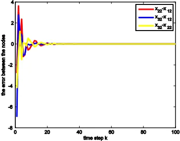
Figure 1: The Synchronization Errors Between The Nodes (The First Entry Of The State)

Figure 2: The Synchronization Errors Between The Nodes (The Second Entry Of The State)

[image:8.612.325.507.490.633.2]

(9)

5. CONCLUSIONS

Efforts have been made to investigate the synchronization problems of an array of coupled discrete-time complex networks subject to nonlinearity, mixed time-delays as well as communication constraints. By choosing a new Lyapunov function, we have derived the criteria under which the investigated complex networks can reach global synchronization in mean square. A numerical example illustrates the effectiveness of the results. Future works will focus on, for example, channels in completely differently adverse communication environments, nodes with complex nonlinear coupling, adaptive controllers design and so on.

REFRENCES:

[1] D.J. Watts, S.H. Strogatz, “Collective dynamics of ’small-world’ network”, Nature, Vol. 393, 1998, pp. 440-442.

[2] A.L. Barab𝑎́si, R. Albert, “Emergence of scaling in random networks”, Science, Vol. 286, 1999, pp. 509-512.

[3] C.G. Li, G.R. Chen, “A comprehensive weighted evolving network model”, Physica A, Vol. 343, 2004, pp. 288-294.

[4] X.F. Wang, G.R. Chen, “Synchronization in small-world dynamical networks”, Int. J. Bifurcat. Chaos, Vol. 12, 2002, pp. 187-192. [5] X.F. Wang, G.R. Chen, “Synchronization in

scale-free dynamical networks: robustness and fragility”, IEEE Trans. CAS-I, Vol. 49, 2002, pp. 54-62.

[6] Y.Q. Yang, X.F. Wu, “Global finite-time synchronization of a class of the non-autonomous chaotic systems”, Nonlinear Dyn, Vol. 70, 2012, pp. 197-208.

[7] C.G. Li, G.R. Chen, “Synchronization in general complex dynamical networks with coupling delays”, Physica A, Vol. 343, 2004, pp. 263-278.

[8] W.L. Lu and T.P. Chen, “Synchronization of Coupled Connected Neural Networks With Delays”, IEEE Trans. Circuits Syst. I, Vol. 51, 2004, pp. 2491-2503.

[9] W.L. Lu and T.P. Chen, “Synchronization analysis of linearly coupled networks of discrete time systems”, Physica D, Vol. 198, 2004, pp. 148-168.

[10] X.D. Li, X.L. Fu, “Lag synchronization of chaotic delayed neural networks via impulsive

control”, IMA J. Math. Control Inform., Vol. 29, 2012, pp. 133-145.

[11] J.L. Wang, H.N. Wu, “Global finite-time synchronization of a class of the non-autonomous chaotic systems”, Nonlinear Dyn, Vol. 70, 2012, pp. 13-24.

[12] J.Y. Cao, G.Z. Wanga, Q.Y. Jianga, Z.X. Han, “A neighbourhood evolving network model”,

Phys. Lett. A, Vol. 349, 2006, pp. 462-466. [13] J.D. Cao, W.W. Yu, Y.Z. Qu, “New complex

network model and convergence dynamical for reputation computation in virtual organizations”, Phys. Lett. A, Vol. 356, 2006, pp. 414-425.

[14] H.J. Gao, J. Lam, G. Chen, “New criteria for synchronization stability of general complex dynamical networks with coupling delays”,

Phys. Lett. A, Vol. 360, 2006, pp. 263-273. [15] C.P. Li, W.G. Sun, J. Kurths, “Synchronization

of complex dynamical networks with time delays”, Physica A, Vol. 361, 2006, pp. 24-34. [16] Z.S. Duan, G.R. Chen, L. Huang,

“Synchronization of weighted networks and complex synchronized regions”, Phys. Lett. A, Vol. 372, 2008, pp. 3741-3751.

[17] Y. Wang, Z.D. Wang, J.L. Liang, “A delay fractioning approach to global synchronization of delayed complex networks with stochastic disturbances”, Phys. Lett. A, Vol. 372, 2008, pp. 6066-6073.

[18] Y.R. Liu, Z.D. Wang, J.L. Liang, X.H. Liu, “Stability and synchronization of discrete-time Markovian jumping neural networks with mixed mode-dependent time delays”, IEEE Trans. Neural Networks, Vol. 20, 2009, pp. 1102-1116. [19] Z.D. Wang, Y. Wang, Y.R. Liu, “Global synchronization for discrete-time stochastic complex networks with randomly occurred nonlinearities and mixed time delays”, IEEE Trans. Neural Networks, Vol. 21, 2010, pp. 11-25.

[20] C.C. Hua, Q.G. Wang, X.P. Guan, “Global adaptive synchronization of complex networks with nonlinear delay coupling”, Phys. Lett. A, Vol. 368, 2007, pp. 281-288.

[21] J. Zhou, J.A. Lu, J.h. L 𝑢̈ , “Adaptive Synchronization of an Uncertain Complex Dynamical Network”, IEEE Trans. Automat. Contr., Vol. 51, 2005, pp. 652-656.

(10)

Man, Cybern. C, Appl. Rev., Vol. 37, 2007, pp. 173-184.

[23] X. He, Z.D. Wang, and D.H. Zhou, “Robust H1 filtering for networked systems with multiple state delays”, Int. J. Control, Vol. 80, 2007, pp. 1217-1232.

[24] G.L. Wei, Z.D. Wang, X. He, H.S. Shu, “Filtering for networked stochastic time-delay systems with sector nonlinearity”, IEEE Trans. Circuits Syst. II, Exp. Briefs, Vol. 56, 2009, pp. 71-75.

[25] J.L. Liang, B. Shen, H.L. Dong, L. James, “Robust distributed state estimation for sensor networks with multiple stochastic communication delays”, Int. J. Sys. Sci., Vol. 9, 2011, pp. 1459-1471.

[26] G.L. Wei, Z.D. Wang, H.S. Shu, “Robust filtering with stochastic nonlinearities and multiple missing measurements”, Automatica, Vol. 45, 2009, pp. 836-841.

[27] H.L. Dong, Z.D. Wang, D. W. C. Ho, H.J. Gao, “Variance-constrained H1 filtering for a class of nonlinear time-varying systems with multiple missing measurements: the finite-horizon case”,

IEEE Trans. Signal Process., Vol. 58, 2010, pp. 2534-2543.

[28] L. Ma, F.P Da, K.J. Zhang, “Exponential 𝐻_∞ filter design for discrete time-delay stochastic systems with Markovian jump parameters and missing measurements”, IEEE Trans. CAS-I, Vol. 58, 2011, pp. 994-1007.