PROCESS DISCOVERY: A NEW METHOD FITTED TO BIG
EVENT LOGS
1
SOUHAIL BOUSHABA, 2MOHAMMAD ISSAM KABBAJ, 3FATIMA-ZAHRA BELOUADHA,4ZOHRA BAKKOURY,
1Ph.D candidate, 2Assistant Professor,3Habilitated Professor, 4Full Professor
AMIPS Research Group, Ecole Mohammadia d’ingénieurs, Mohammed Vth University, Rabat, Morocco E-mail: [email protected], [email protected], [email protected],
4
ABSTRACT
Business process discovery is a research field assembling techniques that allow representation of a business process, taking as input an event log where process data are stored. Several advances have been made in process discovery, but as data volume starts to weight considerably, improvement of discovery methods is crucial to follow up. In this paper, we discuss our new method, inspired from image processing techniques. Adapted to voluminous data logs, our method relies on generation of a Petri net using a matrix representation of data. The principal idea behind our approach consists of using several concepts: partial & feature blocks, filters as well as the adaptation of combinatory logic concepts to process mining in the perspective of extracting a business process model from a big event log.
Keywords: Process Mining, Business Process Management, Process Discovery, Distributed Algorithm
1. INTRODUCTION
Numerous methods, relying on event log exploration, have been elaborated in process discovery. Among these methods, there is a branch that puts more focus on activities’ ordering within a process, for instance, Van der Aalst et. al description of an α-algorithm[1], capable of
describing a large scope of process models. The stated algorithm’s constraint in dealing with short loops and noisy logs was overcome via Medeiros et. al.’s extension of the algorithm to manage short looping [2]. Noise and incompleteness have been dealt with, on the other hand, through more recent algorithms such as fuzzy mining [3] and genetic process mining [4].
Although data quality have been addressed in the algorithms previously mentioned, log volume was poorly considered, which is a challenging obstacle as data stores and therefore event logs tend to grow sustainably. For the sake of quantified records, the United States’ all-sectors confound volume of corporate data averages nearly 200 terabytes per company. On the algorithmic side, the previously mentioned algorithms’ efficiency -when applied to large event logs- was questioned and proved weak by Van der Aalst [5].
Aren’t there any approaches to provide efficient mining of highly voluminous logs?
We discuss in this paper a process discovery algorithm trying to cope with this issue, by the use of matrix representation in block-by-block discovery.
In the remainder of this paper, we first state related works in section 2 then specify the key concepts used in our paper and our approach fundamentals in section 3, the following section investigates block detection, while the fifth section covers pattern type detection. In section 6, we expose our mining process then illustrate our method via a case study in section 7. We conclude our paper and set research perspectives in section 8.
2. RELATED WORKS
Among the discovery algorithms previously written, we state first the α-algorithm [1], which
extracts a considerable set of process models (structured workflow nets, or shortly SWF-nets). Improvements to the algorithm have been made to deal with noise [2] and to discover short loops. The alpha-algorithm has been also conditioned to mine specific Petri-net categories: invisible tasks and non-free choice constraints.
To avoid the volumetric tackle, inductive miner “IM” techniques [13] have been established and lately extended to inductive miner-infrequent “IMi” techniques [14] to cope with behavioral infrequency. The general idea of IM is the extraction of a set of blocks composing the process model by extracting the most relevant design pattern from the directly-follows graphs.
[8] and extended in [15] extracts a set of patterns
from the matrix representation rather than extracting them from a specific (or even, namely most relevant) pattern.
Other works in the field have involved matrix algebra for process representation indeed, Medeiros et. al represent the log of a process as a matrix[9]. This representation -which is not block-oriented-, however, is made through creation of « causal matrix » using the same basic successor operator -direct succession- to inspect the relationship between each pair of tasks in the process.
Matrices were also employed by Chen Li et. Al[10] to represent processes. The authors describe a method to discover a reference process model: from a given set of process variants. Mathematical intuition lacks however to this method as it symbolizes loops by letter L and XOR operator by – as matrix components. We also highlight Chen Li et al.’s method’s input, as it does not operate on the event log itself but on a set of process variants, which induces to ranking the method as a post-process-discovery method [11].
3. KEY CONCEPTS AND APPROACH
FUNDAMENTALS
3.1 Key concepts in data extraction
In order to clear our method’s structure in the reader’s mind, we have to introduce the key concepts that we use: indirect succession operator and characteristic matrix.
Indirect Succession:
Even logs contain traces of successions between tasks, Van der Aalst et. al[1]suggested a direct succession operator, we complete the latter by introducing indirect succession which relies onthe following four basic ordering relations:
• Indirect succession, denoted ⋙
• Causality, denoted ↠
• No succession relationship ≢
• Parallelism, denoted ∥∥
Definition1.Let L be an event log over a set of tasks T and a, b two tasks in T.
a ⋙ b (or a indirectly succeeds b) if and only if there exists a trace σ
t t t . . . t and i, j ∈ 1, . . . , n such that
σ ∈ L, t a, t b and i .
a ↠ bif and only if a ⋙ b and
b ⋙ a.
a ≢ b if and only if a ⋙ b and
b ⋙ a.
a ∥∥ b if and only if a ⋙ b and
b ⋙ a.
For illustration, consider a workflow L=[(A,B,D,E,H), (A,D,C,E,G), (A,C,D,E,G), (A,B,D,E,G), (A,D,B,E,H), (A,C,D,E,H), (A,D,C,E,H)]. We note that:
• A ⋙ H Because there exists a trace (A,B,D,E,H) such that A is indirectly succeeded by H,
• B ≢ C As B is never succeeded by C and C is never succeeded by B.
• D ∥∥ C Because there exists a trace (A,D,C,E,G) where D ⋙ C and there exists a trace (A,C,D,E,G) where C ⋙ D. The following subsection explains how we use only the indirect succession operator to build the characteristic matrix.
Characteristic matrix:
This is a binary matrix that is meant to describe relationships between tasks belonging to a given process, these relationships are detected in event log analysis and the matrix values depend solely on indirect succession between tasks.
Definition2.Let L be an event log composed of traces referring to a set of n tasks denoted#T %∈& .. ', the elements of the matrix are then:
M, 1 if T ⋙ T.
M, 0 otherwise
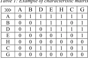
[image:2.595.333.479.499.599.2]The characteristic matrix for the same event log L as extended in the previous subsection is shown in table 1:
Table 1: Example of characteristic matrix
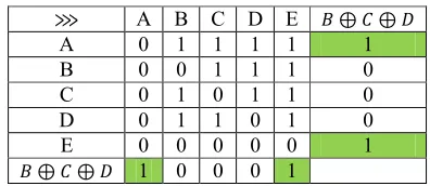
⋙ A B D E H C G A 0 1 1 1 1 1 1 B 0 0 1 1 1 0 1 D 0 1 0 1 1 1 1 E 0 0 0 0 1 0 1 H 0 0 0 0 0 0 0 C 0 0 1 1 1 0 1 G 0 0 0 0 0 0 0
3.2 Approach fundamentals
Figure 1:feature Block successors and predecessors
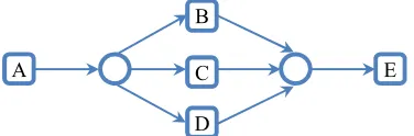
Partial blocks-illustration shown in figure 2- constitute blocks of tasks having a group of common successors and predecessors. We note that each feature block is a partial block but the partial is not necessary a feature block. In the remainder we consider the workflow L = [(A,B,C,D), (A,C,B,D), (A,E,D)] .
Besides, a partial block can be grouped with other tasks to form a feature block. As shown in figures 3, on one hand, {B, E, C} is a feature block (and subsequently, is also considered as partial block). On the other hand, {B, E} and {E, C} are partial blocks. However, grouping {B, E} and {C} generates a parallel feature block. In addition, grouping {A, D} and {B, C, E} generates also a succession feature block that illustrates a complex design pattern representing the global process.
[image:3.595.90.286.352.440.2]Feature block Partial block
Figure 3:Example of block aggregation
4. BLOCK DETECTION
The analysis of design pattern structures synthesis of block detection allowed rules(and filtering). Filters allow detection of both feature and partial blocks and are based on the formalism of each block type as well as the logical similarity operator defined in the next subsection
4.1.Logical Similarity Operator
Once the characteristic matrix is obtained from a set of tasks, the block detection phase is considered to determine whether the selected tasks constitute a feature or partial block. We introduce therefore an operator of logical similarity.
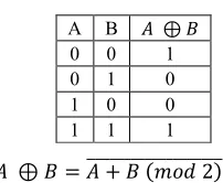
In combinatory logic, the XOR operator results in true whenever both inputs differ (one being true and the other false). Not XOR (symbolized by ⊕) allows then determining whether two Boolean
values are similar or different.
We explicit Not XOR’s formula and establish the operator’s truth table below:
+ ⊕ , + - , #./0 2%2222222222222222222
Our logical similarity operator is to help us verify whether a set of binary n-uples contains the same values. This operator is defined as follows:
Definition3.Let3 &1, 4' and 5 ⊊ 3 with 7890#5% .and let #:;%;∈<be m binary n-uples:
#⨁;∈<:;%>
? @ A @
B 1, CD E :;#./0 .% ;∈<
0
0, CD E :;#./0 .% ;∈<
F 0 ∀C ∈ 3
We note that we consider m binary n-uples#:;%;∈< as m n-uples having the same values if the value of #⨁;∈<:;%> is equal to 1 for any C ∈ 3, according to
the following rule:
Theoreme1. ∀ #:;%;∈<m binary
n-uplesH⊕;∈<:;I #1, … 1%if and only if all #:;%;∈< have the same binary values.
We note that the logical similarity test can be applied to either row or column sets from the characteristic matrix. However, the formulation of
Common predecessors Partial block Common successors
[image:3.595.358.459.385.468.2]Figure 2: Partial Block Common Successors And Predecessors
Table 2: Not Xor Truth Table
[image:3.595.96.279.586.682.2]the similarity output differs slightly:
Definition4.
#⨁;KL M;%>NOPQ
? @ A @
B1 if ES>,;#./0 .% L
;K
0
0 if E S>,;#./0 .% L
;K
F 0
∀ C T &1, 4'
#⨁;KL M;%>UOVWLXQ
? @ A @
B1 if ES;,>#./0 .% L
;K
0
0 if E S;,>#./0 .% L
;K
F 0
∀ C T &1, 4'
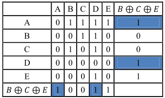
[image:4.595.100.268.340.440.2]We illustrate in Table 3 the results of the cross-similarity test (applied to rows and columns of the matrix described in Table 1)
Table 3: not xor operator applied to rows and columns
A B C D E , ⊕ Y ⊕ Z A 0 1 1 1 1 1 B 0 0 1 1 0 0 C 0 1 0 1 0 0 D 0 0 0 0 0 1 E 0 0 0 1 0 1 , ⊕ Y ⊕ Z 1 0 0 1 1
Our first deduction is that the set {B, C, E} displays a similar behavior to {A, D} blue columns.
4.2.Formalism for blocks
In the previous section, we provided definition to each one of the block types that we encounter in process design patterns. As a reminder, partial blocks contain tasks possessing common successors and predecessors, as per feature blocks; they constitute task blocks having the same successors and the same predecessors among the tasks that are outside their perimeter.
The objective of this subsection is to present formalism that allows clearer and reusable mathematical description of partial & feature block. Consider a set of tasks #T %∈[ ,\] from a given process model. If the set forms a partial block then each task conserves the same behavior keeps towards the remainder of tasks outside the set. In terms of indirect succession, the corresponding matrix elements (outputs of Not XOR cross calculation between block tasks and the rest) must have the same values in rows (respectively in columns).
For the rest of the paper, we will assume that L is a log of n tasks #T % ^ ^ and #M,% ^ , ^ the
corresponding characteristic matrix. Let also
I &1, n'andJ ⊊ I.
We can formalize this criterion of feature blocks by the following definition:
Definition5.The set of the tasks #T %∈a constitute a feature block if and only if:
Have the same values in rows
∀ i, j ∈ J, i b , ∀ c ∈ I\J M,\ M,\ Have the same values in columns
∀ i, j ∈ J, i b , ∀ c ∈ I\J M\, M\,
Direct application of the feature described above to the matrix in Table3 leads to the following results: A selection process applied to the matrix knots must perform application of the property.
Let first consider a random selection of tasks from the process.
The selection forms a feature block if and only if its components display the same behavior towards the non-selected tasks in terms of predecessors and successors. Detection of feature blocks induces therefore calculation of differences and similarities between rows on one hand and columns on the other one. Also, note that calculus can be performed on a distributed grid for each candidate block. We can fit the property mentioned above to our indirect succession operator terminology by the following equivalence:
Theoreme2.The set of the tasks #T %∈aconstitutes a
feature block if and only if:
#⨁∈aT %efgh 1 ∀ j ϵ I\J
#⨁∈aT %jfklm h 1 ∀ j ϵ I\J
According to definition 1, the tasks {B,C,E}form a feature block as they have the same behavior with respect to the other tasks as shown in Table 3 and Table 4 (the value of blue boxes is 1).The set{B,E} is not a feature block because they do not have the same behavior with respect to other tasks as shown in Table 4 (the value of red box is 0).
Table 4:Example of feature blocks
A B C D E BE BCE A 0 1 1 1 1 1 1 B 0 0 1 1 0 1 0 C 0 1 0 1 0 0 0 D 0 0 0 0 0 1 1 E 0 0 0 1 0 1 1 BCE 1 0 0 1 1
We denote by BE the calculus of logical similarity operator:
[image:4.595.335.506.599.693.2]Besides, let’s define three functions SumR, SumC
and TotalS on the space of n-sized binary vectors with values in n:
Definition6.Let #T %∈a the set of the tasks
SumR calculates the number of successors of a given task Ti(we simplify the notation by SumR(i) ). It is the sum of the values corresponding to theith row in the characteristic matrix.
∀ ∈ J, op.q#C% E S;,> >∈<
SumC calculates the number of predecessors of a given task Ti (we simplify the notation by SumC(i) ). It is the sum of the values corresponding to the ith column in the characteristic matrix.
∀ ∈ J, op.Y# % E S>,; >∈<
TotalS returns the number of successors and predecessors of the Crs task. In other words, it sums both SumR and SumC of a given Crsposition
Applying definitions given above, we deduce the following lemma:
Lemma 1.If #M>%>∈<is a feature block then: They have the same number of successors:
∀ C, ∈ 5, C b op.q#C% op.q# %
They have the same number of predecessors:
∀ C, ∈ 5, C b op.Y#C% op.Y# %
They have the same number of predecessors and successors:
∀ C, ∈ 5, C b M/t8uo#C% M/t8uo# %
This is a necessary but not sufficient condition to determine feature blocks. It allows, indeed, to select candidate feature blocks based on the output of calculus on rows and columns of a given block’s matrix representation. Still, candidate blocks are confirmed to be feature blocks only after applying the logical similarity operator. The properties shown in Lemma 1 are meant to simplify feature block detection. Subsequently, we ought to seek a rule to detect feature blocks. The rule is based on the definition below:
Theoreme3.The set of the tasks #M>%>∈<constitutes a feature block if and only if:
∀ C, ∈ 5, C b , M/t8uo#C% M/t8uo# %
and#⨁>∈<M>%;NOPQ 1 ∀ T 3\5
Partial blocks, on the other hand, represent task blocks with a group of common successors and predecessors; the number of successors
&predecessors is not required to be equal for each task from the partial block. It is also worth noting that a feature block is a partial block itself while the other way round is not necessarily true.
According to these findings mentioned above, we define a partial block as follows:
Definition7.Let5 ⊊ 3, v ⊊ 3L and#T %∈a, #T %∈wtwo sets of the tasks where 5 ∩ v ∅ and 5 ∪ v ⊊ 3. The set of the tasks #M>%>∈<constitutes a partial block relative to #M>%>∈{if and only if:
they have the same values in rows
∀ C, ∈ 5 ∪ v, C b , ∀ c ∈ 3#5 ∪ v%S>,| S;,| they have the same values in columns
∀ C, ∈ 5 ∪ v, C b , ∀ c ∈ 3#5 ∪ v%S|,> S|,; Taking account of the number of successors and the predecessors, we can deduce the following lemma if we consider an event log L composed of the set of tasks#T %^ ^ , and the three functions TotalS, SumR and SumC:
Lemma2. Let 5 ⊊ 3, v ⊊ 3L and#T %∈a,
#T %∈wtwo sets of the tasks where 5 ∩ v ∅ and 5 ∪ v ⊊ 3. The set of the tasks
#M>%>∈<constitutes a partial block relative to
#M>%>∈{then:
They have the same number of successors and predecessors
∀ C, ∈ 3 ∪ 5, C b , M/t8uo#C% M/t8uo# %.
Besides, the tasks composing a partial block have the same behavior with respect to a group of tasks in the log. Thus, calculating similarities and differences between rows and columns for a set of tasks in the characteristic matrix help detecting a partial block.
5. PATTERN TYPE DETECTION
We saw previously that the number of successors and predecessors of a block of tasks in a process are properties that shape the block type and also the corresponding design pattern.
In order to answer our main objective, which is process discovery, there are properties to define in the recognition of each one of the covered pattern types.
The design patterns used (succession, XOR and parallel feature patterns) rely here on a set of three activities. Results are generalized to richer task sets and demonstration by recursion is possible.
5.1.Succession Feature Pattern
the adoption of linear functions used in the previous
section (SumR, SumC and TotalS) that operate on the calculus of successors and predecessors. We arrange the linear property in the lemma below:
Lemma 3. Let#M>%>∈<be a set of tasks (sorted by the order of SumR) in a succession feature block with cardinality n then:
∀ C ∈ 5, op.q#C% } 1 op.q#C - 1% ∀ C ∈ 5, op.Y#C% - 1 op.Y#C - 1%
∀ C ∈ 5, M/t8uo#C% 4 } 1
Let’s consider a succession feature pattern of five tasks represented on a Petri net in Figure 4. Let us first consider three tasks out of the set: B, C and D. The characteristic matrix and the successor/predecessor calculus of our sub block BCD are given in Table 5 and Table 6
Figure 4: Example of succession feature pattern
Table 5:Characteristic matrix corresponding to a succession pattern
⋙ B C D SumR B 0 1 1 2 C 0 0 1 1 D 0 0 0 0 SumC 0 1 2
Table 6: Number of successors and predecessors corresponding to an example ofsuccession feature
pattern
SumR SumC TotalS
B 2 0 2
C 1 1 2
D 0 2 2
The results of applying of the logical similarity operator to the characteristic matrix (Table 4) are shown in Table 7. Green-colored boxes show a similar behavior of block BCD with regard to the remnant tasks. Thus, we can say that B, C & D form a feature block.
Table 7:logical similarity operator applied to succession pattern
⋙ A B C D E , ⊕ Y ⊕ ~
A 0 1 1 1 1 1
B 0 0 1 1 1 0
C 0 0 0 1 1 0
D 0 0 0 0 1 1
E 0 0 0 0 0 1
, ⊕ Y ⊕ ~ 1 1 0 0 1
Tasks B, C and D form succession feature block because:
• They have the same behavior towards tasks A and E (note the 1 value in the green cells);
• And the lemma 3 is verified:
o SumR (B) -1 = SumR (C)
o SumC(B)+1 = SumC (C)
o TotalS = 3 - 1 ;
N.B: The verification of SumR and SumC can be verified of each couple of tasks, we take B and C just as an example.
5.2.XOR Feature Pattern
The XOR feature pattern represents a set of tasks running in mutual exclusion.
We set a lemma that allows detection of XOR feature blocks in our approach based on the number of successors and predecessors.
Lemma 4.#M>%>∈<is a set of tasks in a XOR feature block with card(Ti) = n then:
∀ C ∈ 5, op.q#C% 0 ∀ C ∈ 5, op.Y#C% 0 ∀ C ∈ 5, M/t8uo#C% 0
[image:6.595.307.495.546.608.2]Figure 5 illustrates an example of XOR feature pattern presented as a Petri net. The feature block contains tasks B, C and D in mutual exclusion XOR. Its corresponding characteristic matrix and number of successors and predecessors (sum of values of each row and column of its matrix) are respectively given in tables Table 8and Table 9below.
Figure 5: Example of XOR feature pattern
Table 8:characteristic matrix of an example of the XOR feature pattern
⋙ B C D SumR
B 0 0 0 0
C 0 0 0 0
D 0 0 0 0
SumC 0 0 0
A B C D E
A
B
C
D
Table 9:Number of successors and predecessors
corresponding to an example of XOR feature pattern
SumR SumC TotalS
A 0 0 0
B 0 0 0
C 0 0 0
[image:7.595.309.508.249.297.2]We register the results of applying similarity operator to the characteristic matrix in Table 10.
Table 10:Application of similarity operator to XOR feature pattern
⋙ A B C D E , ⊕ Y ⊕ ~ A 0 1 1 1 1 1 B 0 0 0 0 1 1 C 0 0 0 0 1 1 D 0 0 0 0 1 1 E 0 0 0 0 0 1 , ⊕ Y ⊕ ~ 1 1 1 1 1
Tasks B, C and D form an Xor feature block because:
• They have the same behavior towards tasks A and E (note the 1 value in the green bocks);
• And the SumR, SumC & TotalS have the value of 0 (see Table 10);
5.3.Parallel Feature Pattern
Parallel feature pattern regroups tasks running in concurrence. We exploit the same functions operating on successors/predecessors with a specific definition in the lemma below in order to sort a detection criterion to this type of patterns.
Lemma 5.#M>%>∈<is a set of tasks in a parallel feature block with n being the set’s cardinal then:
∀ C ∈ 5, op.q#C% 4 } 1 ∀ C ∈ 5, op.Y#C% 4 } 1 ∀ C ∈ 5, M/t8uo#C% 2 ∗ #4 } 1%
[image:7.595.93.286.253.341.2]Figure 6illustrates an example of parallel feature pattern shown as a Petri net. The feature block is composed of three parallel tasks B, C and D. Its corresponding characteristic matrix and number of successors and predecessors are respectively given in tables Table 11and Table 12.
Figure 6: Example of the parallel feature pattern
Table 11:characteristic matrix for the example of parallel feature pattern
⋙ B C D SumR
B 0 1 1 2
C 1 0 1 2
D 1 1 0 2
SumC 2 2 2
Table 12: Number of successors and predecessors corresponding to the parallel feature pattern
SumR SumC TotalS
B 2 2 4
C 2 2 4
D 2 2 4
Table 13contains results of our sole operator applied to the matrix.
Table 13: logical similarity operator applied to parallel feature pattern
⋙ A B C D E , ⊕ Y ⊕ ~ A 0 1 1 1 1 1 B 0 0 1 1 1 0 C 0 1 0 1 1 0 D 0 1 1 0 1 0 E 0 0 0 0 0 1 , ⊕ Y ⊕ ~ 1 0 0 0 1
Tasks B, C & D form parallel feature block as:
• They have the same behavior regarding tasks A and E (note the 1 value in the green boxes);
• And the:
o SumR = 3-1 = 2
o SumC = 3- 1= 2
o TotalS= 2* (3-1) = 4
6. MINING PROCESS
We define a process model as a set of tasks that respect a design pattern structure. Design patterns can be either basic or complex. The design pattern structure we saw in section 3 contains both partial and feature blocks. By our idea of process mining, we intend to extract these blocks by following mining steps; the proposed method detects start and end blocks of tasks and performs.
The purpose of this section is to present the filters that form the core of our method.
A
B
C D
[image:7.595.307.505.350.436.2] [image:7.595.90.277.658.727.2]6.1.Filter of First and Last Task Detection
To detect the first task, we use a filter based on the following theorems:
Theorem4.The task Tj is the first task if and only if the sum of the corresponding column values of the characteristic matrix equals to minimum of
op.Y# % min>∈• #op.Y#C%%
Detection of the last task requires usage of a filter based on the following theorem with proof below:
Theorem5. The task Tj is the last task if and only if the sum of the corresponding row values of the characteristic matrix equals to min of this value.
op.q# % min>∈• #op.q#C%%
6.2.Mining Algorithm
The input of the mining algorithm is a process event log of a. It extracts the corresponding process model through recursive extractions of feature blocks composing the Petri net representing the process. It is worth noting that the detection of the blocks can be executed on different nodes (the following calculus can be parallelized).
The main steps of the algorithm are the following: first, a characteristic matrix is generated from the event log. Identification of the first and last sets of tasks in the process follows then filters (operating on rows and columns of the matrix) are activated to detect candidate feature and partial blocks. The next step is selection of feature (then partial) blocks using the appropriate filter and testing by logical similarity operator. Discovered feature blocks are masked and replaced by one task in the characteristic matrix. The same iterations are performed considering the new characteristic matrix until a single block is obtained. Note that the detection of a partial block requires detecting the feature blocks composing it (tasks having the same row’s and column’s values), then replacing each one of feature blocks by a unique activity. So, a new candidate feature block is created.
The algorithm is illustrated clearly in the following pseudo-code:
/* Declaration of some used functions Int SumVector (int V[])
{ int S=0 inti=0 Fori=1 to N S=S+V[i] EndFor Return S }
Int[][]ChMatrixBuilder ( int V[]) { int M[][]
/* Application of indirect succession operator to task set
Return M }
Dictionary GroupSelector (intT[],S[]) {
/* Groups tasks by their sum values, returns a dictionary of /* arrays indexed by the distinct values in S.
}
/* Main discovery procedure: Main()
{
/* n is the cardinal of the task set
Const int n
/* i-th task
inti
IntSumR[n],sumCols[n],TotSum[n]
/* These are the row and column vectors
intRi[n], Ci[n]
/* The characteristic matrix.
int M[n][n]
Dictionary Groups, FeatureGroups, FirstTasks, LastTasks
Read T[n]
M=ChMatrixBuilder(T) For i=1 to n
Ri=M.Row(i) Ci=M.Column(i)
/* Calculating and storing the sum of row values for task i
SumR(i)=SumVector(Ri)
/* Calculating and storing the sum of column values for task i
SumCols(i)=SumVector(Ci) TotSum(i)=SumR(i)+SumCols(i) If SumR(i)=0 then
/* We identify first tasks FirstTasks.Add(T(i)) EndIf
If SumCols(i)=0 then /* We identify last tasks LastTasks.Add(T(i)) EndIf
/* building a dictionary containing lists of tasks grouped /* by SumRow, SumCol & TotSum
Groups=GroupSelector(T,Distinct(TotSum))
Fori=1 toGroups.Count
CallComputeSimilarityGroups.key(i)
/* We detect & store feature blocks
FeatureGroups=FeatureGroupDetector(Groups.key (i))
/* We detect & store partial blocks
PartialGroups=PartialGroupDetector(Groups.key(i) )
EndFor
For i=1 to PartialGoup.Count For i=1 to FeatureGroups.Count
Call XOR DetectionFeatureGroups.key(i) Call ParallelDetectionFeatureGroups.key(i) Call SuccessionDetection(FeatureGroups.key(i)
EndFor EndFor
start: Fori=1 toFeatureGroups.Count Call XORDetectionFeatureGroups.key(i) Call ParallelDetectionFeatureGroups.key(i) Call SuccessionDetection(FeatureGroups.key(i) EndFor
/* A procedure that takes the feature
/* block as input and prints its graphical notation
Call Create Petri Net Frame Goto Start
/* A procedure that takes a set of
/* Petri frames and generates graphical aggregation
Call Generate Final Petri Net }
7. CASE STUDY:
[image:9.595.80.519.78.508.2]As a case study, we picked a real process event log [12] as presented in the table below:
Table 14: process event log
Case id Trace
1 (a, b,de,h)
2 (a,d,c,e,g)
3 (a,d,b,e,h)
4 (a,c,d,e,g)
Where:
a = register request, e = decide
b=examine thoroughly g= pay compensation c = examine casually, h = reject request d = check ticket,
We can also denote the log by:
L=[(a,b,d,e,h),(a,d,c,e,g), (a,d,b,e,h), (a,c,d,e,g)] In the reminder of this section, we will present each step performed by our algorithm and its output, when the algorithm is applied to the proposed case study.
Read:
L=[(a,b,d,e,h),(a,d,c,e,g), (a,d,b,e,h), (a,c,d,e,g)] Construct the characteristic matrix:
ComputeSumR and SumC:
Table 15: First characteristic matrix corresponding toL
a b d e h c g SumR a 0 1 1 1 1 1 1 6 b 0 0 1 1 1 0 1 4 d 0 1 0 1 1 1 1 5 e 0 0 0 0 1 0 1 2 h 0 0 0 0 0 0 0 0 c 0 0 1 1 1 0 1 4 g 0 0 0 0 0 0 0 0 SumC 0 2 3 4 5 2 5
Add to First Tasks:{a} because(SumC= min SumC)
Add to Last Tasks: {g , h} because (SumR= min SumR)
ComputeTotalS = SumC +SumR
Table 16: First row and column sums
SumR SumC TotalS
a 6 0 6
b 4 2 6
d 5 3 8
e 2 4 6
h 0 5 5
c 4 2 6
g 0 5 5
Group tasks: {{a,b,e,c},{h,g},{d}}
Compute logical similarity operator to the selected groups
Table17 First logical similarity operator calculus
a b d e h c g
8 ⊕ ‚ ⊕ 7 ⊕ ƒ
„ ⊕ …
a 0 1 1 1 1 1 1 0 1
b 0 0 1 1 1 0 1 0 1
d 0 1 0 1 1 1 1 0 1
e 0 0 0 0 1 0 1 1 1
h 0 0 0 0 0 0 0 1 1
c 0 0 1 1 1 0 1 0 1
g 0 0 0 0 0 0 0 1 1
8 ⊕ ‚ ⊕ 7
⊕ ƒ 1 0 0 0 1 0 1 g⨁h
222222 1 1 1 1 1 1 1
Output:
• The tasks a,b,c, e form a partial block( they have the same behavior only with tasks g and h and not with d “red cells”)
behavior with all other tasks), so it can be
substituted with a unique activity denoted gh Select the tasks having the same row’s value in the partial block {a,b,c,e} which are b and c
[image:10.595.89.287.216.347.2]Compute logical similarity operator to the tasks b and c
Table18First logical similarity operator calculus
a b d e c gh ‚ ⊕ 7
a 0 1 1 1 1 1 1
b 0 0 1 1 0 1 1
d 0 1 0 1 1 1 1
e 0 0 0 0 0 1 1
c 0 0 1 1 0 1 1
gh 0 0 0 0 0 0 1
‚ ⊕ 7 1 1 1 1 1 1
Output:
• The tasks b and c constitute an Xor Partial block
Reduce the characteristic matrix by replacing the feature block with a unique significant activity
Table19 Characteristic matrix after substitution
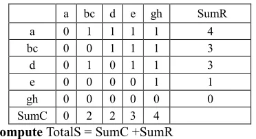
a bc d e gh SumR a 0 1 1 1 1 4 bc 0 0 1 1 1 3 d 0 1 0 1 1 3 e 0 0 0 0 1 1 gh 0 0 0 0 0 0 SumC 0 2 2 3 4
Compute TotalS = SumC +SumR
TABLE 20:FIRST ROW AND COLUMN SUMS
SumR SumC TotalS
a 4 0 4
bc 3 2 5
d 3 2 5
e 1 0 1
gh 0 4 4
Group tasks: {{bc,d},{a,gh},{e}}
[image:10.595.95.281.392.493.2]Compute logical similarity operator to the selected groups
Table 21 Characteristic matrix after substitution
a bc d e gh „… ⊕ 8 ‚7 ⊕ 0 a 0 1 1 1 1 0 1 bc 0 0 1 1 1 0 0 d 0 1 0 1 1 0 0 e 0 0 0 0 1 0 1 gh 0 0 0 0 0 1 1 „… ⊕ 8 0 0 0 0 0
‚7 ⊕ 0 1 0 0 1 1
Output:
• The tasks bc and d form an parallel feature block (blue colored).
• The tasks gh and a are not in block as they
don’t have different behavior with all tasks (blue cells)
Reduce the characteristic matrix by replacing the feature block {bc,d} by a unique significant activity denoted bcd:
Table22 Characteristic matrix after substitution
a bcd e gh a 0 1 1 1 bcd 0 0 1 1 e 0 0 0 1 gh 0 0 0 0 This result represents a succession pattern
Generate a frame of the corresponding process model:
Figure 7: Process model of the case study
[image:10.595.305.510.415.489.2]Recapitulation:
Table 23: recapitulative table
Block Content Nature a a The first task
bcd (b,c),d (b,c) is a parallel block and (b,c),d is a xor block e e Normal succession task gh g,h The final (Xor block)
[image:10.595.310.493.531.587.2]Split the petri net (by replacing each feature block by its components).
Figure 8: Petri net representing the log L
8. CONCLUSION:
In this paper, we presented an algorithmic approach to discover business processes given their event logs. We proceeded first by stating works related to process model discovery notably the α-algorithm and its adaptations to different constraints as loops, data volume. Previous approaches including use of matrix algebra in mining and adaptation of succession operator are discussed. We introduced the key concepts of indirect succession operator and characteristic matrix and explained the fundamentals
[image:10.595.85.295.637.742.2]of our approach of “process models” and “design
pattern structures”. In the following section, we introduced logical similarity operator, explained and illustrated feature and partial block types as well as their mathematical formalism. In pattern type detection we covered XOR, succession and parallel patterns and finally exposed our mining algorithm followed by the case study in the previous section. This work meant to lay the ground to a much complete improvement; In guise of perspectives, we intend to extend pattern discovery to handle loops, we also consider discussion of on-the-fly discovery as data are to be analyzed and process-discovered even before storing in event logs to deal with volume constraint.
We also intend to test our approach using industrial process event logs and to develop a software application to support the algorithm and to provide a quantitative estimation of its performance as compared to other algorithms.
REFRENCES:
[1] W.M.P. van der Aalst, A.J.M.M. Weijters, and L. Maruster “Workflow Mining: Discovering Process Models from Event Logs” IEEE Transactions on Knowledge and Data Engineering,2004 16(9):1128–1142. (IEEE Transactions)
[2] A.K.A. de Medeiros, W.M.P. van der Aalst, and A.J.M.M. Weijters “Workflow Mining: Current Status and Future Directions” In R. Meersman, Z. Tari, and D.C. Schmidt, editors, On the Move to Meaningful Internet Systems 2003: CoopIS, DOA, and ODBASE, volume 2888 of Lecture Notes in Computer Science,2003,pages 389–406. Springer, Berlin.
[3] C.W. Günther and W.M.P. van der Aalst. Fuzzy Mining: Adaptive Process Simplification Based on Multi-Perspective Metrics. In G. Alonso, P. Dadam, and M. Rosemann, editors, International Conference on Business Process Management (BPM 2007), volume 4714 of Lecture Notes in Computer Science2007, pages 328–343. Springer, Berlin. [4] A.K.A de Medeiros, A.J.M.M. Weijters, and
W.M.P. van der Aalst. Genetic Process Mining: An Experimental Evaluation. Data Mining and Knowledge Discovery, 2007 14(2):245–304. [5] Wil M.P. van der Aalst, Desire Lines in Big Data. In
J. Becker and M. Matzner, editors, Promoting Business Process Management Excellence in Russia (PropelleR 2012), 2013pages 23-30. European Research Center for Information Systems,.
[6] Michael Schroeck, Rebecca Shockley, Janet Smart,
Dolores Romero-Morales and Peter Tufano. Analytics: The real-world use of big data 2012 ,IBM Corporation.
[7] A.J.M.M. Weijters and J.T.S. Ribeiro. Flexible Heuristics Miner (FHM). BETA Working Paper Series, WP 334, Eindhoven University of Technology,2010, Eindhoven.
[8] Boushaba, S., Kabbaj, M.I., Bakkoury, Z. Process mining: Matrix representation for bloc discovery, Intelligent Systems: Theories and Applications (SITA), 2013 IEEE.
[9] De Medeiros, A.K.A., Weijters, A.J.M.M., and Van Der Aalst, W.M.P, Using Genetic Algorithms to Mine Process Models: Representation, Operators and Results, 2004, Eindhoven University of Technology, Eindhoven.
[10] Chen, Li. , Manfred, R., and Wombacher, A., Springer Berlin Heidelberg, Discovering Reference Models by Mining Process Variants Using a Heuristic Approach, 2009.
[11] Chen Li, Manfred Reichert, Andreas Wombacher, 2011, Mining Business Process Variants: Challenges, Scenarios, Algorithms, Data & Knowledge Engineering Elsevier,
[12] W.M.P. van der Aalst. Process Mining: Discovery, Conformance and Enhancement of Business Processes,2011 Springer-Verlag, Berlin.
[13] Leemans, S.J.J., Fahland, D., van der Aalst, W.M.P,Discovering block-structured process models from event logs - a constructive approach. In: Petri Nets. Lecture Notes in ComputerScience2013, vol. 7927, pp. 311–329. Springer
[14] Sander J.J. Leemans, Dirk Fahland, and Wil M.P. van der Aalst Discovering Block-Structured Process Models FromEvent Logs Containing Infrequent Behaviour2013. fluxicon.com.