Wavelet based Multi Class image classification
using Neural Network
Ajay Kumar Singh
MITS Deemed University Lakshmangarh, Sikar
Rajasthan, India
Shamik Tiwari
MITS Deemed University Lakshmangarh, Sikar
Rajasthan, India
V.P. Shukla
MITS Deemed University Lakshmangarh, Sikar
Rajasthan, India
ABSTRACT
This paper presents feature extraction and classification of multiclass images by using Haar wavelet transform and back propagation neural network. The wavelet features are extracted from original texture images and corresponding complementary images. The features are made up of different combinations of sub-band images, which offer better discriminating strategy for image classification and enhance the classification rate.
General Terms
Computer Vision, Pattern Recognition
Keywords
Multi class, Wavelet decomposition, Feature Extraction, Neural Network, Haar wavelet
1. INTRODUCTION
Multi class image classification plays an important role in many computer vision applications such as biomedical image processing, automated visual inspection, content based image retrieval, and remote sensing applications. Image classification algorithms can be designed by finding essential features which have strong discriminating power, and training the classifier to classify the image. Scientists and practitioners have made great efforts in developing advanced classification approaches and techniques for improving classification accuracy [1, 2, 3, 4, 5 and 6].
Wavelets are mathematical functions which help in describing the original image into an image in frequency domain, which can further divided into subband images of different frequency components. Each component is studied with a resolution matched to its scale. Wavelet transform has advantages over traditional Fourier method in analyzing physical situations where the signal contains discontinuities and sharp spikes.
In the past two decades, the wavelet transforms are being applied successfully in various applications, such as feature extraction and classification. Wavelet transforms and their variants such as wavelet packets have become an appropriate starting point for classification, especially for texture images [7, 8], due to scale-space localization properties of. Also the choice of filters in the wavelet transform plays an important role in extracting the features of texture images [7, 8].
Neural networks are used as statistical tools in various fields, including Statistics, Engineering, Psychology, Physics and also Economics. The goal of the neural network is to learn or to discover some association between input and output patterns, or to analyze, or to find the structure of the input
patterns. The learning process is achieved through the modification of the connection weights between units. In the work [9] describes multi spectral classification of land-sat images using neural networks. The work in [10] describes the classification of multi spectral remote sensing data using a Back-propagation Neural Network. A comparison to conventional supervised classification by using minimal training set in Artificial Neural Network is given in [11]. Remotely sensed data by using Artificial Neural Network based have been classified in [12] on software package. In [13] different types of noise are classified using feed forward neural network.
In this paper a wavelet feature extraction algorithm is proposed for image classification problem. Here cumulative histograms are generated using different combinations of approximations and detail sub bands of the wavelet decomposed image and then different features are extracted.
This paper is organized as follows: In the next section Wavelet decomposition using Haar wavelet is discussed. Feed Forward Neural Network is discussed in section 3. In section 4 feature extraction algorithm is discussed. Training and classification is discussed in 5 and finally result is discussed in section 6.
2. HAAR WAVELET RANSFORMATION
The Haar transformation technique is used [15] to form a wavelet since it is the simplest wavelet transformation method of all and can effectively serve our interests. In the Haar wavelet transformation method, low-pass filtering is conducted by averaging two adjacent pixel values, whereas the difference between two adjacent pixel values is figured out for high-pass filtering. The Haar wavelet applies a pair of low-pass and high-pass filters to image decomposition first in image columns and then in image rows independently. As a result, it produces four sub-bands as the output of the first level Haar wavelet. The four sub-bands are LL1, HL1, LH1, and HH1. The low-frequency sub-band LL1 can be further decomposed into four sub-bands LL2, HL2, LH2, and HH2 at the next coarser scale. LLi is a reduced resolution corresponding to the low frequency part of the image. The other three sub-bands HLi, LHi and Hhi are the high frequency parts in the vertical, horizontal, and diagonal directions, respectively [8].
The Haar transform cross-multiplies a function against the Haar wavelet with various shifts and stretches, like the Fourier transform cross-multiplies a function against a sine wave with two phases and many stretches. The Haar transform is derived from the Haar matrix. An example of a 4x4 Haar matrix is shown below [16]:
𝐻
4=
1
√4
1
1
1
1
1
1
−1
−1
√2 −√2
0
0
0
0
√2 −√2
3. FEEDFORWARD NEURAL
NETWORK
A successful pattern classification methodology [17] depends heavily on the particular choice of the features used by the classifier .The Back-Propagation is the best known and widely used learning algorithm in training multilayer feed forward neural networks. The feed forward neural net refer to the network consisting of a set of sensory units (source nodes) that constitute the input layer, one or more hidden layers of computation nodes, and an output layer of computation nodes. The input signal propagates through the network in a forward direction, from left to right and on a layer-by-layer basis. Back propagation is a multi-layer feed forward, supervised learning network based on gradient descent learning rule. This BPNN provides a computationally efficient method for changing
the weights in feed forward network, with differentiable activation function units, to learn a training set of input-output data. Being a gradient descent method it minimizes the total squared error of the output computed by the net. The aim is to train the network to achieve a balance between the ability to respond correctly to the input patterns that are used for training and the ability to provide good response to the input that are similar. A typical back propagation network of input layer, one hidden layer and output layer is shown in figure1.
Fig 1: Feed Forward BPN
The steps in the BPN training algorithm are:
Step 1: Initialize the weights.
Step 2: While stopping condition is false, execute step 3 to 10.
Step 3: For each training pair x:t, do steps 4 to 9.
Step 4: Each input unit 𝑋𝑖 , 𝑖 = 1,2, … , 𝑛 receives the input signal, xi and broadcasts it to the next layer.
Step 5: For each hidden layer neuron denoted as 𝑍𝑗, 𝑗 =
1,2, … . , 𝑝.
)
(
inj j i ij i oj injz
f
z
v
x
v
z
Broadcast 𝑧𝑗 to the next layer. Where voj is the bias on j th
hidden unit.
Step 6: For each output neuron 𝑌𝑘, 𝑘 = 1,2, … . 𝑚
ink k j jk j oky
f
y
w
z
w
inky
Step 7: Compute
kfor each output neuron, 𝑌𝑘
1
sin
0 '
z
ce
w
z
w
y
f
y
t
k ok j k jk ink k k k
Where
k is the portion of error correction weight adjustment for wjk i.e. due to an error at the output unit yk,which is back propagated to the hidden unit that feed it into the unit yk and
is learning rate.Step 8: For each hidden neuron
Where
jis the portion of error correction weight adjustment for vij i.e. due to the back propagation of error to the hiddenunit zj
Step 9: Update weights.
ij ij
ij
jk jk
jk
v
old
v
new
v
w
old
w
new
w
)
(
)
(
)
(
)
(
Step 10: Test for stopping condition.
4. METHODOLOGY
Features are the characteristics of the object of interest. Feature extraction methodologies analyze objects and images to extract the most prominent features which are representatives of the various classes of images. Following methodology is used to extract the features of the texture images.
Step 1: Read the RGB image 𝑓(𝑥, 𝑦, 𝑧)
Step 2: Convert the image to gray scale image 𝑓(𝑥, 𝑦).
Step 3: Compute the Haar wavelet coefficients of step2 image, which returns four matrices A, H, V, D corresponding to approximations, horizontal, vertical & diagonal coefficients of image.
Step 4: For each pair of coefficients (A,H), (A,V), (A,D) and
(A-abs(V-H-D)) repeat the step5 to step8.
Suppose first matrix in pair is X & second is Y and get size of
matrix is [M,N].
Step 5: For I=1 to 8 repeat the step 6. Where I represents the 8
neighbors in each direction of any point as shown in figure 2.
Fig 2: 8 neighbors of any point
Step 6: Repeat for J=1 to M Repeat for K=1 to N
d=max(min(X(J,K),Y(I)),min(Y(J,K),X(I))) if d=min(X(J,K))
Set H1(I)=X(J,K) Else
Set H2(I)=Y(J,K) End
End
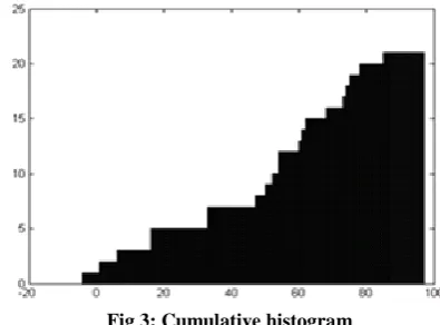
Step 7: For I=1 to 8 cumulative histogram of H1 & H2 is
found shown in the figure 3..
Step 8: For each cumulative histogram correlation
coefficient, mean and standard deviation features are
computed.
Step 9: Repeat step3 to step8 for complement image of
𝑓(𝑥, 𝑦) also.
Step 10: Arrange the features in a matrix.
5. TRAINING AND CLASSIFICATION
In this phase of experiment we have divided each texture image in to sixteen blocks of equal size, out of which six blocks are used as samples to train the neural classifier and remaining ten blocks are used as samples to test the texture class. Texture features are extracted using the algorithm discussed in part 4 for each of the six samples.
[image:3.595.325.523.215.361.2]Fig 3: Cumulative histogram
Then neural classifier is trained with this feature set. After training the classifier random samples for test are selected for classification. Features of these samples are also extracted using the same feature extraction algorithm discussed in part 4, and applied to neural classifier for testing.
The classification is performed over a 5-10-15 feed forward neural network model that consist of one input layer with five neurons, one hidden layer with ten neurons and one output layer with fifteen neurons. Back propagation is pertained as network training principle where the training dataset is constructed by the extracted features of the image. The entire input features are normalized into the range of [0,1], whereas the output class is assigned to one for the highest probability and zero for the lowest.
6. EXPERIMENTAL RESULT
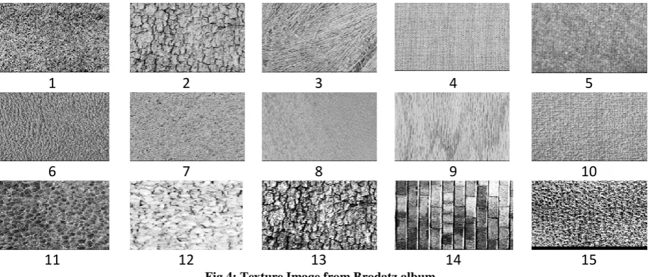
6.1 Data Set
1
2
3
4
5
6
7
8
9
10
[image:4.595.72.532.70.265.2]11
12
13
14
15
Fig 4: Texture Image from Brodatz album
S.No. Texture
Montiel et al. (2005)
Proposed System
1 Grass (D9) 99.06 98.56
2 Bark (D12) 100 100
3 Straw (D15) 100 100
4 Herringbone weave
(D15) Not Tested 86.02
5 Woolen cloth (D19) Not Tested 95.6
6 Pressed calf leather
(D24) 100 100
7 Beach sand (D29) 85 90.8
8 Water (D38) 100 100
9 Wood grain (D68) 100 98.8
10 Raffia (D84) 100 96.8
11 Plastic bubbles(D112) Not Tested 86.4
12 Gravel Not Tested 99.06
13 Field Stone 76.25 85.25
14 Brickwall Not Tested 95.45
15 Pigskin (D92 H.E.) 92.5 91.56
Table 1: Comparison of result
6.2 Feature Extraction
Features are computed with the algorithm discussed in section iv of a block. This process generates 384 features (2 images ( 1 original + 1 complement) *4 combinations ((A,H),(A,V), (A,D), (A, abs(V-H-D)))* 3 features (correlation coefficient, mean and standard deviation)*16 histograms. This forms a feature vector of 90 blocks of a single category. Then a feature matrix of fifteen categories is prepared to train the neural network. Similarly a feature vector for test blocks is calculated.
6.3 Classification Results
The experiments were conducted using neural network and the results are shown in Table 1 which compares performance of the classification produced by binary feature selection [18]. Feature extraction method in this paper has boosted the performance in the Beach sand texture by 5.8 percent. Performance is also improved in Field stone texture. The proposed system is simple and computationally less expensive
than the method in [18], which employs computationally expensive genetic algorithm. Our experiments also include some new textures Herringbone, Woolen cloth, Plastic bubbles, Gravel and Brickwall.
7. CONCLUSION
In the proposed image classification system we have introduced new approach using Haar wavelet decomposition and Back Propagation Neural Network. We used the correlation coefficient, mean and standard deviation features of the various combinations of coefficients produced by the wavelet transform. A number of texture images not considered in the work [18] have been analyzed in this work and have been found working within the range 86.2- 99.06% of the performance. This work may further be extended with feature extraction using curvelet and ridgelet transform.
8. ACKNOWLEDGEMENT
The authors would like to thank Faculty of Engineering & Technology of Mody Institute of Technology & Science, Lakshmangarh for providing necessary facilities to carry out this research work.
9. REFERENCES
[1] Gong, P. and Howarth, P.J.,”Frequency-based contextual classification and gray-level vector reduction for land-use identification” Photogrammetric Engineering and Remote Sensing, 58, pp. 423–437. 1992.
[2] Kontoes C., Wilkinson G.G., Burrill A., Goffredo, S. and Megier J, “An experimental system for the integration of GIS data in knowledge-based image analysis for remote sensing of agriculture” International Journal of Geographical Information Systems, 7, pp. 247–262, 1993.
[3] Foody G.M., ”Approaches for the production and evaluation of fuzzy land cover classification from remotely-sensed data” International Journal of Remote Sensing, 17,pp. 1317–1340 1996.
[5] Aplin P., Atkinson P.M. and Curran P.J,” Per-field classification of land use using the forthcoming very fine spatial resolution satellite sensors: problems and potential solutions” Advances in Remote Sensing and GIS Analysis, pp. 219–239,1999.
[6] Stuckens J., Coppin P.R. and Bauer, M.E.,”Integrating contextual information with per-pixel classification for improved land cover classification” Remote Sensing of Environment, 71, pp. 282–296, 2000.
[7] Mojsilovic A., Popovic M.V. and D. M. Rackov, “On the selection of an optimal wavelet basis for texture characterization”, IEEE Transactions on Image Processing, vol. 9, pp. 2043–2050, December 2000.
[8] M. Unser, “Texture classification and segmentation using wavelets frames”, IEEE Transactions on Image Processing, vol. 4, pp. 1549–1560, November 1995.
[9] Bishop H., Schneider, W. Pinz A.J., “Multispectral classification of Landsat –images using Neural Network”, IEEE Transactions on Geo Science and Remote Sensing. 30(3), 482-490, 1992.
[10] Heerman.P.D.and Khazenie, “Classification of multi spectral remote sensing data using a back propagation neural network”, IEEE trans. Geosci. Remote Sensing, 30(1),81-88,1992.
[11] Hepner.G.F., “Artificial Neural Network classification using minimal training set: comparision to conventional supervised classification” Photogrammetric Engineering and Remote Sensing, 56,469-473,1990.
[12] Mohanty.k.k. and Majumbar. T.J.,”An Artificial Neural Network (ANN) based software package for classification of remotely sensed data”, Computers and Geosciences, 81-87, 1996.
[13] Shamik Tiwari, Ajay Kumar Singh and V P Shukla, “Statistical Moments based Noise Classification using Feed Forward Back Propagation Neural Network”, International Journal of Computer Applications 18(2):36-40, March 2011.
[14] Stéphane G. Mallat, 1999, “A wavelet tour of signal processing”, Academic Press, 1999.
[15] Chin-Chen Chang, Jun-Chou Chuang and Yih-Shin Hu, “Similar Image Retrieval Based On Wavelet Transformation, International Journal Of Wavelets”, Multiresolution And Information Processing, Vol. 2, No. 2, 2004, pp.111–120, 2004.
[16] Charles K. Chui, “An Introduction to Wavelets”, Academic Press, 1992.
[17] Kumar S., ”Neural Networks: A Classroom Approach”, 1st Edn., Tata Mc-Graw Hill Publications, ISBN: 0-07-048292-6, pp: 169,2004.
[18] Montiel E., Aguado A. S., M. S. Nixon, “Texture classification via conditional histograms”, Pattern Recognition Letters, 26, pp. 1740-1751(2005).