Application of Local Linear Wavelet Neural Network in Short Term Electric Load Forecasting

ABSTRACT

The electrical deregulated market increases the need for short-term load forecast algorithms in order to assists electrical utilities in activities such as planning , operating and controlling electric energy systems. Methodologies based on regression methods have been widely used with satisfactory results. However, this type of approach has some shortcomings. This paper proposes a short- term load forecast methodology based on Artificial Intelligence techniques. The work presented in this paper makes use of local linear wavelet neural networks (LLWNN) to find the electric load for a given period, with a certain confidence level.

General Terms

Electric load, Forecast, Gradient descent. Local Linear Wavelet Neural Network (LLWNN).

Keywords

Wavelet neural network (WNN), artificial neural network (ANN), artificial intelligence (AI), Weekly mean absolute percentage error (WMAPE).

1. INTRODUCTION

Electric load forecasting is used by power companies to anticipate the amount of power needed to supply the demand. In the last few years, various techniques for the STLF have been proposed and applied to power systems. Conventional methods based on time series analysis exploit the inherent relationship between the present hour load, weather variables and the past hour load. Auto regressive (AR) and moving average (MA) and mixed Auto regressive moving average (ARMA) models [1] are prominent in the time series approach. The main disadvantage is that these models require complex modeling techniques and heavy computational effort to produce reasonably accurate results [2]. Basically, most of statistical methods are based on linear analysis. Since the electric load is non linear function of its input features, the behavior of electric load signal can not completely be captured by the statistical methods. So statistical methods are not adaptive to rapid load variations. Another difficulty lies in estimating and adjusting the model parameters, which are estimated from historical data that may not reveal short term load pattern change [3]. The emergence of artificial intelligence (AI) techniques has led to their application in STLF as expert system type models. These methods are discrete and logical in nature. By simply learning the historical samples, these methods can map the input-output relations and then can be used for the prediction.

Among the AI techniques available, different models of NNs due to flexibility in data modeling have received great deal of attention by the researchers in the area of STLF.

.Many type of NN models which are characterized by their topology and learning rules have been successfully used for STLF problems [4]-[14]. A comprehensive review of the literature on the application of NNs to the load forecasting can be found in [9].

Another useful technique for STLF, proposed in the recent years is wavelet based NN method. In this method wavelet is merged with NN and termed as wavelet neural network (WNN). The WNN has been emerged as a powerful new type of ANN. But the major drawback of the WNN is that for higher dimensional problems many hidden layer units are needed. Curse of dimensionality is an unsolved problem in WNN theory which brings some difficulties in applying the WNN to high dimensional problem. So the applications of WNN are usually limited to problems of small input dimensions. The main reason is that they are composed of regularly dilated and translated wavelets. The number of wavelets in the WNN drastically increases with the dimension.

In order to take the advantages of local capacity of the wavelet basic function while not having too many hidden units, the architecture of LLWNN has been used in this paper for STLF. To the best of the authors’ knowledge, a Local Linear Wavelet Neural Network (LLWNN) has not yet been tested for electric load forecasting. In this paper an LLWNN model which smoothly maps the input-output space by adapting the shape of wavelet basis function of hidden layer neurons according to training data set is examined for electric load prediction of the Ontario electricity market. The proposed model does not require external decomposer/composer. So risk of loosing high frequency components of electric load signal is averted. It is found that prediction of electric load based on LLWNN model gives better performance because of its favorable property of modeling the non-stationary high frequency signals such as electric load.

The rest of the paper is organized as follows: Section 2 describes main characteristics of the electric load series. Architecture of LLWNN is described in section 3. Training of LLWNN model by standard BP gradient descent algorithm is described in section 4. Section 5 describes the statistical measures used to evaluate the forecasting performance. Section 6 presents results and discussions on electric load forecast of Ontario electricity market. Finally, section 7. provides concluding remarks.

Application of Local Linear Wavelet Neural Network in

Short Term Electric Load Forecasting

Prasanta Kumar Pany S. P. Ghoshal

National Institute of Technology. National Institute of Technology

Durgapur Durgapur West Bengal, India. West Bengal, India

2. LOAD-DATA ANALYSIS

To develop an appropriate model for load forecasting, we examine the main characteristics of the hourly load series in this Section. To illustrate the forecasting procedure the electric load for the Ontario electricity market from 1st April 2009 to 31st December, 2009 is used for prediction. According to the data samples for each hour of the day and each day of the month, it is clear that the load dynamics have multiple seasonal patterns, corresponding to a daily and weekly periodicity, respectively, and are also influenced by a calendar effect, i.e. weekends and holidays.

It can be observed that the load series presents multiple periodicities and hence, the past load demand could affect and imply the future load demand. If load at hour h (dh) is to be forecasted, the load information of previous hours up to “m” hours i.e.

d

_h1,

d

_h2,

...

d

_hm should

be taken as a part of the input of short term load forecasting (STLF) model. The auto co-relation function (ACF) can be used to identify the degree of association between data in the load series separated by different time lags i.e. previous load. The historical hourly data of 7 days prior to the day whose load to be predicted have been considered to build the forecasting model. Hence the total data points are equal to 7 x 24 = 168. Since the proposed model uses price data 7

hours ago to predict the price

d

_h,168-7=161 input vectors are used to develop the forecast model.

3

.

ARCHITECTURE OF LLWNN

The LLWNN model for the hourly Ontario electric load is developed to forecast for three time periods. The first period comprises two consequent weeks from April 24 to May 7, 2009. The second period contains two weeks from August 25 to September 7, 2009 and the last period includes two weeks, starting on October 9 and ending on October 22, 2009. The historical hourly load data to construct LLWNN model which would be employed to forecast the load data of test week are shown in table 1.

TABLE 1

Hourly load data for forecasting model construction and testing

Seasons Historical hourly load data

Test weeks

Summer April 24-30,2009 May 1-7,2009

Rainy

August25-31,2009

Sept. 1-7,2009

Winter Oct. 9-15,2009 Oct. 16-22,2009

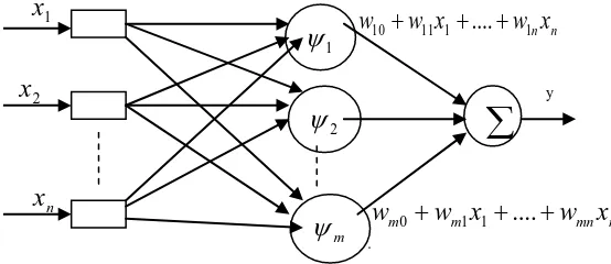
The structure of LLWNN model is shown in Fig. 1. It comprises of input layer, hidden layer and linear output layer. The input data in input layer of the network are directly transmitted into the wavelet layer. As the hidden layer neurons make use of wavelets as activation functions, these neurons are usually called ‘wavelons’. . In stead of using multi layered neural networks and its several variants, a LLWNN is used for forecasting the next day and next week electric load in a deregulated environment.

. In the proposed model, one hour ahead load forecasting using seven hours before load data and twenty four hours ahead forecasting using seven days i.e. 168 hours before load data have been used.

According to wavelet transformation theory, wavelets in the following form is a family of functions, generated from one single function ψ(x) by the operation of dilation and translation ψ(x), which is localized in both time space and the frequency space , is called a mother wavelet



a

b

R

i

z



a

b

x

a

_{i i} n

i i i

i















 







1/2



:

,

,



……… (1)

)

,...

,

(

x

₁

x

₂

x

_n

x



)

,...

,

(

_{i1 i2 in}

i

a

a

a

a



)

...

,

(

_{i1 i2 in}

i

b

b

b

b



The parameters

a

_i and

b

_i are the scale and translation parameters, respectively. According to the previous researches, the two parameters can either be predetermined based on wavelet transformation theory or be determined by a training algorithm.

In the standard form of wavelet neural network, the output of a WNN is given by



z

i

R

b

a

a

b

x

a

w

x

w

x

f

_{i i}

i i i

m

i i m

i i

i















 















(

)

:

,

,

)

(

1/2

1 1





(2) The above wavelet neural network is a kind of basis function neural network in the sense of that the wavelet consists of the basis function. An intrinsic feature of the basis function networks is the localized activation of the hidden layer units, so that the connection weights associated with the units can be viewed as locally accurate piecewise constant models whose validity for a given input is indicated by the activation functions. Compared to the multilayer perceptron neural network, this local capacity provides some advantages such as the learning efficiency and the structure transparency. However, the problem of basis function networks is also led by it. Due to the crudeness of the local approximation, a large number of basis function units have to be employed to approximate a given system. A shortcoming of the wavelet neural network is that for higher dimensional problems many hidden layer units are needed. In order to take advantage of the local capacity of the wavelet basis functions while not having too many hidden units, LLWNN has been used as an alternative neural network.

The difference of a local linear wavelet neural network (LLWNN) with conventional wavelet neural network (WNN) is that the connection weights between the hidden layer and output layer of conventional WNN are replaced by a local linear model. The output of LLWNN is given by













m

i

i n in i

i

w

x

w

x

x

w

Y

1

1 1

0

...

)

(

)

(



(3)

The mother wavelet is

i)



(

x

)



2

2

2

2



x

e

x





(4)

ii)

2

)

(

       







c x

e

where x =

d

₁2



d

₂2



...



d

_n2

Instead of the straight forward weight wi (piecewise constant

model), a linear model

n in i

i

i

w

w

x

w

x

v



₀



_{1 1}



...



is introduced.

The activities of the linear models

v

_i(i=1,2,---n) are determined by the associated locally active wavelet functions ψi(x) (i= 1,2,---,n), thus

v

i is only locally

significant .Non-linear wavelet basis functions (named wavelets) are localized in both time space and frequency space.

Fig.1 – General structure of a local linear wavelet neural network.

4.

TRAINING

A neural learning algorithm to get all the unknown parameters of network i.e. translation and dilation coefficients, weights may be used for supervised training of an LLWNN. Since the function computed by the LLWNN model is differentiable with respect all the mentioned unknown parameters, a standard back propagation (BP) gradient descent training algorithm can be used for updating weights, dilation, translation parameters which are randomly initialized at beginning. The trained LLWNN would be used to predict the hourly load for the next day.

It is possible to over fit the training data if the training session is not stopped at the right point. The unset of the over fitting can be detected through cross validation in which the available data set are divided in to training, validation and testing subsets. The training set is used to compute the gradients and update all the unknown parameters of the networks. The error on the validation set is monitored during the training session. In this work, the standard BP gradient algorithm has been adopted. Training is based on minimization of the cost function (E), given as:

2

10 1 11 1 1 20 2 21 1 2

0 1 1

( ) ( ) ... ( ) ( ) ... 1

2 ... m m( ) m m ... mn n m( )

d w x w d x w x w d x

E

w x w d w d x

   

  

     

 

  _{   } 

 

2

(6)

Where‘d’ is the desired load Gradient descent method for updating the parameters:

w

E

e

k

w

k

w











1

)

(

)



(

.(7)

such that

w

₁₀

(

k



1

)



w

₁₀

(

k

)





e



₁

(

x

)

w

₁₁

(

k



1)



w

₁₁

( )

k



 

ed

_{1 1}

( )

x

and so on Similarly,



















k

e

E

k

1

)

(

)

(

(8)

c

E

e

k

c

k

c











1

)

(

)



(

(9)

Such that

1

1 1 10 11 1 1

1

( )

(

k

1)

( )

k

e w

(

w d

...

w d

_{n n}

)



x











 











(10)

1 1 1 10 11 1 1

1 ( ( )) ( 1) ( ) ( ... n n)

x

c k c k e w w d w d

c



 

     



(11)

2 1 2

3 4

1 1

(

))

(









x

e

x

x











(12)

 

2 2 1

2 3

1 1

1

(

)

2

(

)









x c

e

c

x

x



 







(13)

2

2 1 1 1

1 1

1

)

(

4

))

(

(

_  _













x c

e

x

c

c

x

(14)

5

. ACCURACY

MEASURES

Mean absolute percentage error (MAPE) is used to assess prediction accuracy of the developed models in the paper. The absolute error (AE) is defined as

1



2



m





y

n n

x

w

x

w

w

₁₀



_{11 1}



....



₁

.

n mn m

m

w

x

w

x

w

0



1 1



....



.

1

x

2

x

[image:3.595.77.354.237.357.2]

,

,

,

_{f t}

t

a t

da t

d

AE

d





(15)

The daily mean absolute error (DMAE) can become computed as follows.

DMAE =





24

1

24

1

t t

AE

(16)

The daily mean absolute percentage error

(DMAPE) =





24

1

24

100

t t

AE

(17)

The weekly mean absolute error

(WMAE) =





168

1

168

1

t t

AE

(18)

And,

The weekly mean absolute percentage error

(WMAPE) =





168

1

168

100

t t

AE

(1 9)

6

. RESULTS &

ANALYSIS

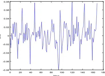
The historical data of Ontario System load from May 2009to December 2009 was used for testing the proposed LLWNN model. The forecasted load obtained with proposed model during summer test week is shown in Fig.2 along with actual load and the corresponding error is shown in Fig. 3.

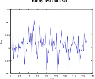
. The forecasted load obtained with proposed Model during rainy test week is shown in Fig.4 along with actual load and the corresponding error is shown in Fig. 5.

. The forecasted price obtained with proposed Model during winter test week is shown in Fig.6 along with actual load and the corresponding error is shown in Fig. 7.

It can be seen from figures that the predicated electricity load of the test weeks are quite close to the actual one. The weekly MAPEs of the generated forecasts, using the models developed in this paper for the three seasons under study, are presented in Table 2.

For comparison purposes, the weekly MAPEs of the generated forecast, using linear regression method (PM1), non linear regression method (PM2), nonparametric regression model (PM3), partial least square regression model (PM4), [15] are also presented in table 2.

TABLE 2Comparison between statistical tools and proposed model for DMAPE of a typical week in the different seasons of the year 2009.

Days in different seasons

PM 1 PM 2 PM 3 PM 4 LLWNN

1-7 May, 09

8.2 8.3 8.0 7.9 7.2897

1-7 Sept.,09

6.4 6.6 6.9 6.6 6.7831

16-22 Oct.,09

9.8 9.6 10.4 10.3 6.0191

Accuracy of LLWNN model is better than the other models in 1st and 3rd time periods. Overall, accuracy of LLWNN model is also better than the other models.

The best results were achieved for 3rd time period.

Figures 2, 4, 6 and table 3 give the comparison result of the output of the dynamic system and output of the LLWNN and the identification error. The relative errors for the training data set and test data set of 3rd time period taking d_data as input vectors in proposed model by using gradient descent algorithm as learning algorithm, where d_data=(load data-minimum load)/(maximum load-data-minimum load) for a given period are represented in table 3. These results in uneven accuracy distribution throughout the week that reflects reality. Thus the results of proposed model show significant improvement in the electric load forecasting process.

TABLE -3

Results obtained by proposed model for 1st 24 hours of a day of 1st and 3rd time periods.

For 1st period test data set For 3rd period test data set

Predicted hourly load taking d_data as input vector

Hourly Error

Predicted hourly load taking d_data as input vector

Hourly Error

0.4376 0.4676 0.4420 0.4543 0.4509 0.4111 0.4268 0.4150 0.4319 0.4670 0.4403 0.4168 0.4439 0.4820 0.4339 0.2973 0.2422 0.1935 0.1688 0.1567 0.1558 0.1785 0.2288 0.3366

-0.0063 -0.0286 0.0055 0.0008 -0.0101 0.0274 0.0045 0.0240 0.0314 -0.0029 0.0062 0.0303 0.0289 - 0.0164 -0.0542 -0.0071 -0.0203 -0.0042 0.0049 0.0050 0.0012 0.0027 0.0504 0.0638

0.4701 0.4780 0.5177 0.5242 0.5417 0.5533 0.4846 0.4121 0.3949 0.2431 0.2211 0.2195 0.1739 0.1778 0.2027 0.2667 0.3833 0.5158 0.4964 0.4970 0.5049 0.4852 0.4657 0.4684

0.0217 0.0355 0.0149 0.0287 0.0271 -0.0144 - 0.0076 -0.0092 - 0.0440 0.0012 0.0002 -0.0222 0.0160 0.0160 0.0323 0.0691 0.0780 -0.0177 0.0088 0.0072 -0.0068 0.0025 0.0178 0.0057

7

.

CONCLUSION

LLWNN model since both smooth global sharp local variation of electric load signal can be effectively represented by the wavelet basis activation function for hidden layer neuron without any decomposer/composer. This method averts the risk of loosing the high frequency components of electric load signals.

8

.

ACKNOWLEDGMENTS

The authors would like to thank the experts who have contributed towards development of the template.

9

.

REFERENCES

[1] S.J.Huang and K.R.Shih.Short term load forecasting via ARMA model identification including non-Guassian process consideration, IEEE Trans. On power systems, vol 18,no 2, pp 673-679,may 2003..

[2] I.Maghram and S.Rahman:. Analysis and evaluation of five short term load forecasting techniques IEEE Trans. On power systems, pp 1484-1491, Apr 1989.

[3] S.Rahman, O. Hazim. Generalized knowledge based short term load forecasting technique, IEEE Trans. On power systems, vol. 8,no 2,pp508-514, May 1993.

[4] C.N.Lu and S.Vemuri. Neural network based short term load forecasting, IEEE Trans. On power systems, vol 8, no.1, pp336-342, Feb 1993.

[5] T.W.S Chow and C.T. Leung. Non-linear autoregressive integrated neural network model for short term load forecasting, IEE proc. Generation transmission and distribution, vol. 143, no.5, pp500-506, Sep 1996.

[6] R.Lamedica,A Prudenzi, M Sforna, M.Caciotta and V.O Cancels. Neural network based technique for short term forecasting of anomalous load periods, IEEE Trans. On power systems, vol 11 no. 4, pp 1749-1756,Nov 1996..

[7] I.Drezga and S.Rahman. Short term load forecasting with local ANN predictors, IEEE Tran. On power systems, vol 14, no. 3, pp 844-850, Aug 1999.

[8] H.Chen, C.Canizare, and A. Singh. ANN based short term load forecasting in electricity markets, proc. IEEE winter meeting, Columbus, Ohio, 2, pp 411-415, Jan 2001.

[9] H.S.Hippert, C.E.Pedreira and R.C. Souza, Neural network for short term load forecasting, a review and evaluation, IEEE trans. On power systems, vol. 16, no.1, pp 44-55, Feb 2001.

[10]T.Senjya, H. Takara, K.Uezato and T. Funabashi. One hour ahead load forecasting using neural network, IEEE trans. On power systems, Vol. 17, no.1, pp 113-118, 2002.

[11]J.W.Taylor and R.Buizza, Neural network load forecasting with weather ensemble predictors, IEEE Transactions on Power systems, pp. 626-632, Aug 2002.

[12]L.M.Saini and M.K Soni. Artificial neural network based peak load forecasting using conjugate gradient methods, IEEE Transactions on Power Systems, vol 12, no.3, pp. 907-912, Aug 2002.

[13]P.Mandal, T. Sanjyu, N.urasaki and T. Funabashi. A neural. Network based several hour ahead electric load forecasting using similar days approach. Int. Journal of electric power and energy system, vol 28, no 6, pp367-373, Jul 2006.

[14]D.Benaouda, F. Murtagh, J.L. Stark and O.Renaud, Wavelet based non linear multiscale decomposition model for electricity load forecasting, Neuro computing vol 70, pp 139-154, dec 2006.

[15]S. M.Kelo, S.V. Dudul.Short Term load prediction with a special emphasis on weather compensation using a novel committee of wavelet recurrent neural networks and regression methods, IEEE, 2010.

0 20 40 60 80 100 120 140 160 180 0

0.2 0.4 0.6 0.8

Hour

P

re

di

ct

ed

Te

st

lo

ad

0 20 40 60 80 100 120 140 160 180 0

0.2 0.4 0.6 0.8

Hour

Te

st

lo

ad

F Fig.2 Dynamic system output and model output for su summer test data set

0 20 40 60 80 100 120 140 160 180

-0.08 -0.06 -0.04 -0.02 0 0.02 0.04 0.06 0.08

Hour

E

rr

or

Fig.3. Hourly error for summer test data set.

0 20 40 60 80 100 120 140 160 180

0 0.2 0.4 0.6 0.8

Hour

P

re

di

ct

ed

Te

st

lo

ad

0 20 40 60 80 100 120 140 160 180

0 0.5 1

Hour

Te

st

lo

[image:5.595.317.500.425.558.2]

ad

Rainy test data set

0 20 40 60 80 100 120 140 160 180 -0.1

-0.05 0 0.05 0.1 0.15

Hour

E

rr

[image:6.595.90.279.76.234.2]

or

Fig-5 Hourly error for Rainy test data set

0 20 40 60 80 100 120 140 160 180 0

0.2 0.4 0.6 0.8

Hour

P

re

di

ct

ed

Te

st

lo

ad

0 20 40 60 80 100 120 140 160 180 0

0.2 0.4 0.6 0.8

Hour

Te

st

lo

[image:6.595.119.305.280.427.2]

ad

Fig-6 Dynamic system output and model output for winter test data set

0 20 40 60 80 100 120 140 160 180 -0.06

-0.04 -0.02 0 0.02 0.04 0.06 0.08 0.1

Hour

E

rr

[image:6.595.96.363.466.662.2]

or

Fig-7 Hourly error for winter test data set -0.20 100 200 300 400 500 600 700 800 -0.15

-0.1 -0.05 0 0.05 0.1 0.15

Hour

E

rr

o

r

0 100 200 300 400 500 600 700 800 0

0.5 1 1.5

Hour

P

re

d

ic

te

d

l

o

a

d

0 100 200 300 400 500 600 700 800 0

0.5 1 1.5

Hour

Tr

a

in

in

g

l

o

a

d

0 20 40 60 80 100 120 140 160 180 -0.2

-0.1 0 0.1 0.2 0.3 0.4 0.5

Hour

er

ro