Intergenerational Long Term Effects of Preschool Structural Estimates from a Discrete Dynamic Programming Model

Munich Personal RePEc Archive

Intergenerational Long Term Effects of

Preschool - Structural Estimates from a

Discrete Dynamic Programming Model

Heckman, James and Raut, Lakshmi

27 January 2002

Online at

https://mpra.ub.uni-muenchen.de/20657/

Intergenerational Long Term Effects of Preschool

-Structural Estimates from a Discrete Dynamic

Programming Model

∗

James J. Heckman Department of Economics

University of Chicago Chicago, IL 60637 mailto:[email protected]

Lakshmi K. Raut† Social Security Administration

500 E Street, SW, 9th_Floor Washington, DC 20254 mailto:[email protected]

Abstract

Using the NLSY79 and the NLSY79 Children and Young Adults datasets, this paper formulates, provides conditions for parametric and non-parametric identification and empirically estimates the parameters of an altruistic model of parental preschool investment within a structural dynamic programming framework. It then examines the effect of a publicly provided preschool policy to disadvantaged children on their educational and labor market achievements, and also on the inter-generational long-term effects on social mobility, college mobility, and earnings inequality. The paper calculates the tax burden of such a social contract policy, taking into account these intra- and inter-generational effects.

Keywords: Preschool Investment, Early Childhood Development, Intergenerational Social Mobility, Structural Dynamic Programming

JEL Classification Nos.: J24, J62, O15, I21

First Draft: December 2002

This Draft: December 2009

∗_{An earlier draft was presented at the Western Economic Association Meeting, 2007, University of Southern}

California, Indian Statistical Institute, The University of Nevada at Las Vegas, and California State University at Fullerton. Comments of the participants of these workshops, especially of Juan Pantano as a discussant of the Western Economic Association conference are gratefully acknowledged

†_{Corresponding author. Raut is an Economist at the Social Security Administration (SSA). This paper}

Intergenerational Long Term Effects of Preschool

-Structural Estimates from a Discrete Dynamic

Programming Model

1

Introduction

We formulate an altruistic model of parental preschool investment within a structural stochas-tic dynamic programming framework. The structural parameters of a structural dynamic programming model are, in general, not all statistically identified (see Hansen and Sargent (1981), and Rust (1994)). If some parameters are not identified, the estimation of these pa-rameters using the maximum likelihood estimation procedure or any other optimizing pro-cedures may cause serious computational problems. Moreover, the policy analysis based on unidentified parameter estimates is of very little content. In this paper we provide con-ditions for parametric and non-parametric identification of our structural dynamic program-ming model, estimate the structural parameters using the maximum likelihood estimation procedure, and then use these estimated parameters to examine the effect of preschool on the production of cognitive and non-cognitive skills of children, their effects on school and labor market achievements, and the intergenerational long-term effects on social mobility, schooling mobility and earnings inequality.

In the past three decades, the income gap between the rich and the poor and the wage gap between the college educated and the non-college educated workers in the US have been widening. Equalizing education has remained as the main policy in the US to reduce poverty and income disparities. Many are, however, highly skeptical about a positive answer to the basic question: ”Can we conquer poverty through school?”

There are many reasons for this skepticism. In the US, education up to high school level is virtually free. Yet many children of poor SES do not complete high school and many of them perform poorly in schools. This naturally beckons to the possibility that the poor quality of the public schools that the children of poor SES attend is the reason for such failings. Improving school quality will improve school performance of these children only marginally. Many empirical studies find that better school quality in terms of lower class size, higher public expenditures per pupil, improved curriculum, and higher desegregation have only marginal effects on school performance of the children of poor SES. See Hanushek (1986) for a survey of the studies along this line.

Taub, 2002), among researchers in economics (see for instance, Heckman, 2000 and Currie, 2001, Cunha, Heckman, Lochner and Masterov, 2006) and among researchers in sociology, psychology and education (see for in stance, Barnett, 1995, Entwisle, 1995, McCormick, 1989, Schweinhart et al., 1993) that children of poor SES are not prepared for college be-cause they were not prepared for school to begin with. The most effective intervention for the children of poor SES should be directed at the preschool stage so that these children are prepared for school and college. The question is then, does the preschool has long-term positive effects on school performance and labor market success? This is the main issue that we address in this paper.

There are two types of quantitative studies on this issue. One set of studies use data on high cost high quality pilot preschool programs such as the High Scope/Perry Preschool Program and the North Carolina Abecedarian Study. These studies find a substantial lasting effect of these programs on school performance and labor market outcomes. The partici-pants in these programs are, however, a very small in number and are not representative of the US population.

The other set of studies use data on the Head Start preschool program which is funded by the Federal government. It is available to the children whose parents earn incomes below poverty line. Not all eligible children are, however, covered by the program. The quality of the program is very poor compared to the above mentioned pilot programs or most private preschool programs. Some studies find that the Head Start Preschool Program has no long-term effect on children's cognitive achievements and school performance, especially for black children. Currie and Thomas (1995) carry out a careful econometric investigation and conclude that the benefits disappear for black children because most of the Head Start black children attend low quality public schools. But after controlling for the school quality, they find significant positive effects of Head Start Preschool Program. See Barnett (1995) for a survey of other studies on the long-term school effect of early childhood programs.

education level, innate ability, and family background. Heckman and Rubinstein (2001) used data on GED testing program in the US, after careful econometric analysis they show that non-cognitive skills are important determinant of earnings and educational attainment. The rest of the paper is organized as follows. Section 2 provides the basic decision making framework. Section 3 defines notations of the paper. Section 4 develops the inter-generational altruism model of parental preschool investment within a structural dynamic programming framework. Section 5 deals with the issues related to identification of the structural parameters of the dynamic programming model. Section 6 describes the estima-tion algorithm that we use. Secestima-tion 7 provides the empirical specificaestima-tions of the producestima-tion processes of cognitive and non-cognitive skills and reports the parameter estimates. Section 8 carries out policy analysis. Section 9 concludes the paper.

2

The Basic Framework

In this section we formulate an econometrically implementable model of preschool invest-ment decision of an altruistic parent in a dynamic programming framework. The preschool investment decision of a parent depends on several other decisions at later stages of a child's life. While we describe each of these decision stages for a better understanding of our frame-work and for future frame-work, in this paper, however, we restrict only to preschool investment decision, taking all other decisions as exogenously given. We treat each parent-child pair as independent. We assume parthenogenetic mode of biological reproduction in our model and with due respect to both genders, we address all individuals in male gender.

2.1

Individual Decision Problem

We assume that an individual's life comprises of several discrete periods during which im-portant life-cycle events relevant to leaning and earning occur. While it may be more real-istic to have finer divisions of these periods, for analytical tractability and given data limita-tions, we aggregate the whole life-cycle into four periods: [0-5), [5-17), [17-26), [26--]. In each of these periods some educational and labor market decisions are made and outcomes are observed.

self-esteem skill, η, and internal self-control skill φ. The levels of these skills that a child

develop depend on various other childhood interventions, for instance, on the child-rearing practices at home, the nature of neighborhood and home environments in which the child grows up (see Mohanty and Raut, 2009 for more on this), and the level of schooling, cog-nitive, socialization and motivational skills of the parent. We do not, however, explicitly include these additional determinants of skill formation in this paper to keep computations manageable.

During ages [5-17), the child goes to school. The school performance at this stage de-pends on his level ofτ,σ,µ,η,andφthat the child has acquired during the previous stage,

on the quality of the school that he attends1_{, and the type of neighborhood kids whom the} child mingles with. It also depends on the parental home inputs such as how many hours the parent spend time with the child to do his homework, how many hours the child watches TV, and how stable and stimulating the relationships among the family members are. Many of these are choice variables for the parent. We do not have adequate information about these factors in our dataset, so we do not include them.

During ages [17-26), the child decides whether to complete college education or not, which depends on his parent's income, his learned and innate abilities. We take this decision as exogenously given, and denote it as the functions(τ,σ,µ,η,φ, s,ε_s),whereε_srepresents

the random events during the life-cycle of the child that affect his schooling decision. During ages [26-], he works, forms his family, has one child and decides how much to invest in his child's preschool. We assume that apart from the level of schooling, and other cognitive and non-cognitive skills, there are other life cycle events and variation in tastes that affect individual's choices. We bundle all these unobserved sources of heterogeneity among individuals into a vector of random variablesε.The state variables of our system are

represented by the vectorz = (τ,σ,µ,η,φ, s,ε). We denote the observable components of

the state variable byx = (τ,σ,µ,η,φ, s)and use the notationz = (x,ε).For any variable

w,we adopt the convention of usingwif it refers to a parent andw′ _{if it refers to his child.}

We assume that given his parental preschool investment decision a, and a realization of his parent's state variablesz = (x,ε), the components of a child's state variablez′ ₌

(x′_,ε′_{), wherex}′ _{= (τ}′_,σ′_,µ′_,η′_,ϕ′_),andε′ _{are generated stochastically by the following}

1_{See Nishimura and Raut (2007) for a model of parental choice of school quality in an altruistic dynamic}

conditional probability density functions:

qτ

(

dτ′|τ, s, a)

(1) qσ

(

dσ′|τ′,τ,σ,µ, s, a)

qµ

(

dµ′|τ′,τ,σ,µ, s, a)

qη

(

dη′|τ′,τ,σ,µ, s, a)

qϕ

(

dϕ′|τ′,τ,σ,µ, s, a)

qs(ds′|τ′,σ′,µ′, s, a)

g(

dε′|τ′,σ′,µ′, s′)

In the above specifications of the conditional probabilities, the conditioning variables conform to what we know in the child development literature about the production processes of these state variables. We will discuss the details of each production process in section 7.2. Given the density functions in Eq. (1), the transition probability densityp(dx′, dε′|x,ε, a)

over the states of our system is determined.

We assume that the lifetime average annualized permanent earnings of an individual with the state variable(x,ε)is represented by an earning functionw(x,ε). Let Abe the set of all possible preschool investment choices of a parent. We assume it to be an ordered set. Assume that the annualized average cost to a parent of making a preschool investment choice a isθ(a), a ∈ A. Given his choicea and permanent annualized income w, the

annualized permanent consumption c(w, a) is then given by c(w, a) ≡ w−θ(a).The

choices of a parent with observable characteristics x are restricted to the set A(x,ε) ≡ {a ∈ A|c(w(x,ε), a)>0}. The choicea yields direct utility from life-time annualized

consumption and indirect utility through its effect on child outcomes and welfare, as repre-sented in the following Bellman equation corresponding to the parent's preschool investment decision problem

V(x,ε) = max

a∈A(x,ε)u(x,ε, a) +β

∫

V(

x′_,ε′)

p(

dx′_{, dε}′_{|x,ε, a}) (2)

whereV(.)is the intergenerational welfare function, known in the dynamic programming

literature as the value function,u(.)is the felicity index of yearly permanent consumption

over the whole lifetime of the parent, and the parameterβmeasures the degree of parental

altruism toward the child.

Under general regularity conditions on u(.), p(dx′, dε′|x,ε, a)andβ, the value

Bhat-tacharya and Majumdar, 1989, Theorem 3.2). Given u(.), p(dx′, dε′|x,ε, a)and β,

sat-isfying the regularity conditions, we carry out a Lucas-Critique free policy evaluation by examining a policy's effect on the individual optimal decisiona,on the intergenerational welfare levelV, and we also examine the intergenerational long-run aggregate effect of the policy on the economy by aggregating individual choices with respect to the long-run pop-ulation distribution, also known as the invariant poppop-ulation distribution, of the equilibrium transition probability distributionp(dx′, dε′|x,ε, a∗(x,ε)).

To be able to do this, we need to estimate the structural parameters. Our data consists of a sample of parent-child pairs with information on parent's observable state x,child's observable statex′_{,parent's permanent incomew,and the parent's preschool investment}

de-cisiona.Suppose a vector of parametersξ_pspecifies the probability distributions in Eq. (1),

i.e., givenξ_p,the transition probability distribution p(dx′, dε′|x,ε, a)is determined. Our

problem is then to statistically estimate the structural parametersζ ={u(.),ξ_p,β}given

observable information on a random sample of parent-child pairsy ={(x_i, x_i′), a_i}n_i=1such

that the predicted behaviors of the sample from the model are close to observed behavior. We denote the log-likelihood function of the sample by L_y(ζ). Estimation of the model involves two steps: For a givenζ, calculate the probability distribution of the endogenous

variablesa_i|x_iandx′

i|xi, aiusing the model to form the log-likelihood of the sampleLy(ζ)

and then use an appropriate estimation procedure to choose aζ.

Two questions need be addressed to that end. First, is the computation of the likelihood

L_y(ζ),which involves solving the dynamic programming problem in Eq. (2) repeatedly for

each(x,ε), feasible with the currently available computing technology, especially whenε

is a continuous multivariate random variable? Second, are the structural parameters of the model identified (the definition of identification is stated later)?

The answer to both questions is in general no. Following the literature, we make sim-plifying assumptions to transform the above structural dynamic programming problem into a random utility model of discrete choices. We will show that these assumptions greatly simplify the computation and the identification of the structural parameters of the model. Given those assumptions, we will see two facts: First, the set of structural parametersξ_p

determines the transition distributionp(x′_{|x, a)of the observable state variables, which is}

the mixture distribution of the original transition probability distribution, more specifically p(x′|x, a) =∫

p(x′,ε′|x,ε, a) dε|x dε′|x′. Second, the set of optimal choice probabilities

P(a|x), a∈ A(x), x∈ Xover the observed discrete choices depends onξ_ponly through

Notice that the optimal choiceais treated as an exogenous variable in the estimation of p(x′|x, a),the maximization of joint likelihood of two components is more efficient. To

make estimation task computationally manageable, however, again following the trend in the literature, in place ofξ_p, we take an estimate of p(x′|x, a)as our fixed parameters in

the vector of parametersζ,and in place of β,we calibrate βfrom other information, and

then form the likelihood of the sample of observed discrete choicesai|xi for identification

and estimation of the remaining parameters.

3

Notation

In the rest of the paper, our parameter vector isζ ={u(x, a), p(x′|x, a),β},a∈ A(x), x ∈

Xwherep(x′|x, a)andβare fixed. Denote byΞthe set of all such parameter values. We de-note byL_y(ζ)the log-likelihood of the sample of observed choicesy={a_i|xi, i =1...n}.

Given a set of conditional choice probabilities{P(a|x), a∈ A(x), x ∈X}which depends

onζ,the log-likelihood functionL_y(ζ)of the sample is defined.

Let Jxdenote the number of elements in the feasible choice set A(x). Denote byJ =

∑_x∈XJ_x.Assume thatXis a finite ordered set ofMelements.

Denote by F(a) = [f(x′|x, a)]_x′_,x∈X the Jx× Jx′ conditional transition probability

matrix given a choicea∈ A(x)where the element f(x′|x, a)corresponding to the rowx

and the columnx′ _{is the probability of the child moving to statex}′ _{given that his parent is}

from the statexand he had made a choicea∈ A(x).We denote byF(x, a)the row vector

ofF(a)corresponding to the parent's statex.

The vector of conditional choice probabilities denoted byP ={P(a|x), a∈ A(x), x ∈X}

is ordered by the primary index of ordering inXand the secondary index of the ordering in A. For eachx,the component vector of conditional choice probabilities{P(a|x), a∈ A(x)}

belongs to aJx−1dimensional simplex. The set of all vectorsPof conditional choice

prob-abilities△is a subset ofℜMJ₊₊which is restricted to the interior of theM-fold cross product

of theJx−1dimensional simplices.

For any functionv(x, a),its vector representation is aJ×1vectorv(i.e., with the same

symbolv) in which the function valuesv(x, a)'s are ordered in the same way as inP. For

any scalar or a vector functionw(x),we denote byw(again using the same symbolwto

denote it) the values ofwstacked in rows in the same order as in the ordered setX. For any random vector or a random variablew(x, a),we denote its expectation with

wis a random vector, the product inside this summation is element-by-element). Define the M×JmatrixΠderived from a vector of conditional choice probabilitiesPby

Π

M×J =





P(a=1|x₁) ... P(a= J|x₁) ... 0 ... 0

0 ... 0 ... 0 ... 0

0 ... 0 ... P(a=1|x_M) ... P(a = J|x_M)





and the transition matrices in matrix notation as aJ×MmatrixFby,

F

J×M =

         

f(x′₁|x₁, a=1) ... f(x′_M|x₁, a=1)

...

f(x′₁|x1, a= Jx1) ... f(x′M|x1, a= Jx1)

... f(x′

1|xM, a=1) ... f(x′M|xM, a=1)

...

f(x′₁|x_M, a= J_xM) ... f(x′_M|x_M, a= J_xM)

         

4

Structural Estimation

The structural estimation of the original problem is computationally intractable. Similar to Rust (1994), we make the following simplifying assumptions to transform the original model in Eq. (1) to a random utility model. In the next two sections, we utilize these simplifications to find conditions for identification and estimation of structural parameters. We assume that w(x,ε)and hence A(x,ε)does not depend onε, i.e.,w()does not

contain any unobservable idiosyncratic shocks. However, we assume that ε represents a

taste shifter for individual preferences and constitutes our only source of unobserved het-erogeneity, the specific nature of which is stated formally in the following assumption.

Assumption 1

alla∈ A(x).

We also make the following additional assumptions.

Assumption 2

some twice continuously differentiable density functiongwith finite first moment.

Assumption 3

x1_{, ..x}M}

Under assumptions 1 - 3 , we have

V(x,ε) = max

a∈A(x)u(x, a) +ε(a) +β_x

∑

∫

V(

x′_,ε′)

g(

dε′|x′)

f(

x′_{|x, a})

(3)

Denote the value function, after integrating out the unobservable component of the state variable, byv(x)≡∫

V(x,ε)g(dε|x). Integrating both sides of Equation (3) with respect

to the conditional densityg(dε|x), and utilizing this notation forv(x), we have

v(x) =

∫

max

a∈A [˜v(x, a) +ε(a)]g(dε|x) (4)

where

˜v(x, a) ≡ u(x, a) +β

∑

x′_∈X

v(

x′)

f(

x′_{|x, a})

(5)

= u(x, a) +βF(x, a).v

Eq. (4) above is a random utility model in which the function ˜v(x, a)measures the common

utility that an individual of observable characteristicsx derives from a choicea ∈ A(x).

Denote by

Ω(x, a) ={

ε|˜v(x, a) +ε(a)≥ ˜v(

x, a′)

+ε(a′),for alla′ ∈ A(x)}

(6)

the set of individuals with observed characteristicsxwho made aas their optimal choice. The conditional choice probabilities are then given by

P(a|x) =

∫

Ω(x,a)g(dε|x). (7)

By partitioning the domain of integral in Eq. (4) into disjoint regionsΩ(x, a), a∈ A(x), x ∈

Xand then integrating we have the following,

v(x) =

∑

P(a|x)

[

u(x, a) +

∫

Ω(x,a)ε(a)g(dε|x)

P(a|x) +β_x

∑

v(

x′)

f(

x′_{|x, a}) ]

=

∑

P(a|x) [u(x, a) +e(x, a) +βF(x, a)·v] ...(*) (8)

= ¯u(x) +¯e(x) +β¯F(x)·v

where

e(x, a)≡

∫

in line (*) is the conditional expectation of the componentε(a)of the random vectorεgiven

xanda.Writing the above in matrix notation, we have

v= ¯u+ ¯e+β¯F·v≡Φ(v,ζ) (10)

Letv(ζ)be a fixed point of the mapΦ(v,ζ)for givenζ ∈ Ξ,and denote byP(v)the

conditional choice probabilities in Eq. (7) for a given value functionv. Then the computa-tion of the likelihood of the sample is simplified to the computacomputa-tion of the fixed point of the above mapΦ(v,ζ).The computation ofP(a|x),ande(x, a)involve multi-dimensional

numerical integration, which may make computations extremely slow. Both computational tasks are, however, substantially simplified under the following assumption:

Assumption 4

as extreme value distribution with location parameter 0 and scale parameter 1.

McFadden (1981) has shown that under Assumption 4, e(x, a) = (λ−ln P(a|x)),

whereλis the Euler-Mascheroni constant, with a numerical value ofλ=0.57721566, and

the conditional choice probabilityP(a|x)has the following Logit representation,

P(a|x) = e˜v (x,a)

∑_a∈De˜v(x,a′) (11)

The above strategy of computational simplification was pioneered by Rust (1987). The computational burdens could be, however, further simplified as follows: From Eq. (10) it follows thatv= [I_M−β¯F]−1[¯u+¯e].Substituting this in Eq. (5), we have

˜v(x, a) =u(x, a) +βF(x, a) [I_M−β¯F]−1[¯u+¯e] (12)

It is easy to see that givenP₀∈△, the right hand side of the above, and hence, a new vector of

conditional choice probabilities sayP₁∈△can easily be computed by substituting it in Eq.

(11). We represent this relationship for each structural parameterζ ∈ ΞbyP₁= Ψ₍P₀,ζ).

Following the line of argument in Aguirregabiria and Mira (2002), it is easy to show that for eachζ ∈ Ξ,there exists a unique fixed pointP(ζ)to the mappingΨ(P,ζ),and starting

from any initialP₀∈△, the iterative processP_n+1 = Ψ(Pn,ζ), n ≥ 0converges to the

fixed pointP(ζ)∈△. Thus, for each structural parameter ζ ∈ Ξ,there exists a unique likelihood of the sampleL_y(ζ),the computation of which is brought down to computation

5

Identification of Structural Parameters

In the previous section we saw that givenζ ∈ Ξ,there exists a unique likelihood function

L_y(ζ). To be able to estimateζ ∈ Ξ_,the model should be identified in the sense that

L_y(ζ) =L_y(

ζ′)a.e.if and only ifζ = ζ′, (13)

the a.e. is with respect to the dominant probability measure defining the likelihood of the sample. Following Prakasa Rao (1992), we say that our model isglobally identifiedif the relationship in Eq. (13) holds for any twoζ,ζ′ ∈Ξ,and islocally identifiedaround a partic-ular parameterζ ∈ Ξ,if the relationship in Eq. (13) holds for allζ′ ∈Ξin a neighborhood ofζ.

To find reasonable conditions for identification, from Eq. (6) note that the optimal choices are invariant if we add a locationmxand divide both sides by a scale factorσx >0,

for eachx∈ X.Thus it follows that we can recover the utility function only up to a scale and location. Given this fact, we restrict the one period utility function(u(x, a), a∈ A(x))to

lie in aJx−1dimensional open submanifold ofℜJx for eachx∈ X. We take each possible

utility vector(u(x, a), a∈ A(x), x ∈X)to lie in the cross product (or equivalently in the

direct sum, if we viewℜJx to be embedded in_ℜJ) of theseJ_x−1dimensional submanifolds

over allx ∈ X. There are many such manifolds, and up to diffeomorphisms they are all

equivalent. We define one such manifoldU using the mapϕ:△ ∋ P 7→u∈ ℜJ (which

reads as,ϕtakes a memberP in△to a memberuinℜJ) by

u=[IJ+βF(IM−β¯F)−1Π]−1_[˜v−˜e]≡ ϕ(P) (14)

where ˜v(x, a) =ln P(a|x)and ˜e= βF(IM−β¯F)−1Πe.TakeU = ϕ−1(△).It can be

shown that the setU is a J−M dimensional smooth manifold. Given parametersβ,and

Ffixed, we restrict our parameter spaceΞto be such that theu-component of a parameter vector ζ ∈ Ξ is restricted to lie in U. The most general non-parametric family that we

can restrict our parameters u to lie in is U. Our nonparametric identification issue boils

down to the question, under what conditions can we identify our structural model in this non-parametric family ofU? Theorem 1 addresses this, using the following assumption

Note that there always exist such β′s at least near β = 0. Also note thatβ = 1 will

violate condition (2) since in that caseIM−β¯Fis not invertible, as each row will add-up to

zero.

Theorem 1 (

Nonparametric Identification)

Fof the parameter vectors are fixed. LetP ∈ △be a vector of conditional choice

probabili-ties that satisfy Assumption 5. Then there exists a unique utility function(u(x, a), a∈ A(x), x∈ X)

∈ U that generatesP as the optimal solution to the choice problem in Eq. (2).

Further-more, the model in Eq. (2) is globally or locally non-parametrically identified depending on whether Assumption 5 holds globally or locally.

Proof.LetP ∈ △be a vector of conditional choice probabilities that satisfy Assumption 5.

Note that writing Eq. (12) in matrix notation, we have ˜v= [I_J+βF(I_M−β¯F)−1Π]u+

βF(I_M−β¯F)−1Πe,where ¯Fis the expectation ofF(a)with respect toP. Taking ˜v(x, a)≡

ln P(a|x),and denoting by ˜e=βF(I_M−β¯F)−1Πe,we have

u=[I_J+βF(I_M−β¯F)−1Π]−1[˜v− ˜e] (15)

Thus by Assumption 5, for eachP, there exists a uniqueu∈ U.

We now prove the second part regarding the nonparametric identification. Note that the data on distribution of choices given a fixed number of individuals n(x) (a positive

integer) for each observed value of individual characteristicsx ∈ Xcan be summarized as

an ordered vectorydefined similar toPbyy= (n(a|x), a∈ A(x), x ∈X)wheren(a|x)

is the number of individuals who chosea ∈ A(x)given their characteristics x ∈ X. The

likelihood of the sample can be written as follows

Ly(P) =

∏

n(x)!

∏_a∈A(x)n_a(x)!exp

(

∑

(x)ln

(

1−

Jx−1

∑

(a|x)

))

×

exp

(

∑

Jx−1

∑

n(a|x)ln

(

P(a|x)

1−∑_aJx₌−₁1P(a|x)

))

= h(y)g(η)exp(

y′_η)

, whereη= (η(a|x), a∈ A(x), x∈ X),with

η(a|x) = ln

(

P(a|x)

1−∑_aJx₌−₁1P(a|x)

)

,andg(η) =−

_∑

(

1+

Jx−1

∑

η(a|x)

)

,

andh(y)is the multiplicative component in the first expression. It follows from the above

thatLy(P)is an exponential distribution. The determinant det(I_(P))of the Fisher

det(I_{(P)) =} [

∏_x∈X∏_aJx₌−₁1P(a|x)]−1,which is always > 0since each P(a|x) > 0.

Since det(I_(P))is a continuous function of _P, there exists a neighborhood of _P in _△

such that the Fisher information matrix is of full rank for allPin that neighborhood.

More-over, note that the functiong(η)is continuously differentiable inη.Hence by Prakash Rao

(1992, Theorem 6.3.2), for any P′ in a neighborhood of P, we have L_y(P) = L_y(P′)

a.e. ⇔ P =P′. But u = ϕ(P) in Eq. (14) is a 1-1 function from △ to U around P ∈ △ that satisfies Assumption 5. Hence for anyζ ∈ Ξsuch that the corresponding

P(ζ)satisfies Assumption 5, there exists a neighborhood ofζ inΞsuch that for anyζ′in

that neighborhood,Ly(P(ζ)) = Ly(P(ζ′))a.e. ⇔ζ =ζ′.Hence the model in Eq. (2)

is locally nonparametrically identified around aζwhose associatedP(ζ)satisfies

Assump-tion 5. It is also clear that if AssumpAssump-tion 5 is true for allP ∈ △, the model in Eq. (2) is

also globally identified.

The conditional choice probabilitiesP ={P(a|x), a∈ A, x∈X}are nothing but the

aggregate demand functions of discrete choicesa ∈ Aas a function of individual

charac-teristicsx∈ X. The characteristicsx ∈Xis acting like a price of the Marshallian demand

function. Nonparametric identification problem in our set-up can be viewed as the well-known aggregation problem of the consumer theory: Given a system of demand functions

P ∈ △, when does there exist a utility functionu(x, a)that generates P as the optimal

solution of problem in Eq. (2)? The above theorem provides conditions for an analogous aggregation problem in the present context of structural dynamic programming problem.

Suppose instead of most general non-parametric utility specifications for the parameter vectorζ, we parametrizeu(and also possiblyβ, but Fis still assumed to be fixed) to have

a parametric formζ :Θ→ Ξ,whereΘ⊂ ℜk,k < J−M+1is an open set. When can

we identify such parametric models? To state our sufficient condition for this, we recall a definition from the Differential Geometry. A map f :Θ → △is an immersionatθ ∈

Θ, an open subset ofℜk, if the differential mapd fθ : ℜk → Tf(θ)(△)is injective, i.e.,

one-to-one, whereTf(θ)(△)is the tangent space of the manifold△at f(θ).

Theorem 2 (

Parametric Identification)

model is globally identified if and only if the mapP(ζ(θ))is an injective map.

L_y(P(ζ(θ))) = L_y(

P(

ζ(

θ′)))a.e. implies

P(ζ(θ)) = P(

ζ(

θ′))since

L_y(P)is

globally identified in the parameter space△by theorem 1. Henceθ = θ′ sinceP(ζ(θ))

is 1-1 in this neighborhood. The second part follows immediately.

6

Econometric implementation

The structural estimation of discrete dynamic programming models has two components. One component involves solving a fixed point problem associated with the dynamic pro-gramming problem to compute the likelihood function of the sample, and the second com-ponent involves finding a set of structural parameters to maximize the likelihood of the sample. Rust (1987) used a fixed point algorithm on value function, and then used the value function to compute the optimal choice probabilities for each set of structural parameters. Whereas, Hotz and Miller (1993) used the fixed point algorithm on the choice probabilities and then used these choice probabilities to compute the value function. Both procedures then carried the likelihood maximization to find an estimate of the structural parameters. Aguirregabiria and Mira (2002) introduced a faster estimation procedure by interchanging the order of executing these two components of the computation. They showed that their estimation procedure has good asymptotic properties. Our estimation procedure follows the Aguirregabiria and Mira procedure which can be briefly described as follows: First we computeF, the transition probability matrix, from the subset of the data of the type(x_i, x_i′)

of the observable states for all parent-child pairs. We then assume a parametric form of the utility functionuθ(x, a),whereθ∈ ℜk and follow these steps:

1. Start with an initial J×1vector of probabilitiesP₀ ∈ △.

2. Maximize the likelihoodL(θ;P₀) =

∏

P0(ai|xi,θ),where

P(a_i|x_i,θ) = e˜v (x,a;θ)

∑_a∈De˜v(x,a′;θ)

˜v(x, a) = uθ(x, a) +βF(x, a) [IM−β¯F]−1[¯uθ+ ¯e]

3. Givenθ∗in step 2, computeP₁= (P(a|x,θ∗), x∈ X, a∈ A)∈ △from the above

formula.

Following Aguirregabiria and Mira (2002), we parameterizeuθ(x, a) =θ0w(x)−θ1a,

whereθ₀is the marginal utility of annualized lifetime earnings, andθ₁/θ₀is the preschool

investment cost in the unit of earningsw. Note thatuθ(x, a)is not identified, because for

eachx∈ X,the ordered vector(uθ(x, a), a∈ A(x))should belong to an one dimensional

subspace ofℜ2,in this specificationulies in a two-dimensional manifold instead. However,

the parameter measuring the preschool investment costθ₁/θ0is identified.

We have used the public domain Sun Java programming language to implement the above estimation procedure and for all other computational tasks.

7

Empirical Findings

7.1

The Dataset and Variables

For our analysis we use the NLSY79 dataset and the NLSY79 Children and Young Adults. The NLSY79 dataset contains a nationally representative sample of 12,686 young men and women who were 14-22 years old when they were first surveyed in 1979, i.e., these sampled individuals represent a population born in the 1950s and 1960s, and living in the United States in 1979. These individuals are interviewed annually. The dataset has records of school and labor market experiences of these individuals and also the information on their cognitive and non-cognitive traits. We, however, also need information on most of these variables for the parents of the respondents. This dataset does not have much information on respondents' parents. So we link this dataset with the NLSY79 Children and Young Adults dataset. The child survey dataset includes longitudinal assessments of each child's cognitive, attitudinal and social, motivational, academic and labor market experiences.

Two other important datasets in this area of research are the High/Scope Perry Preschool Study and the Carolina Abecedarian Project. These are small scale pilot programs with small number of participants. Data from these programs contain school performance information but the labor market outcome data is weak. While these datasets are good for studying the effect of high quality preschool program on school performance and labor market success, these datasets do not nationally representative samples, because the participants were selec-tively chosen. For details on the High/Scope Perry Preschool Study see Schweinhart et al. (1993) and on the Abecedarian Project, see Campbell et al. (1998).

the labor market outcomes to a child's preschool experiences regarding the child rearing methods, home environment, teaching methods followed in schools. While the dataset con-tains the school performance of these children, the sampled cohorts will have data on labor market outcomes available only many years later in the future.

7.2

Production of non-cognitive skills

We show in the next two subsections that non-cognitive skills are important determinants of earnings and learning. In this section we consider the production process of these skills. The literature in sociology, psychology, early childhood development and physiology suggest that early childhood investment is the most crucial input for development of cog-nitive and non-cogcog-nitive skills. The studies in these literatures link school success to home environment, child rearing practices, neighborhood type in which the kid is raised. For in-stance, the Coleman report (1966) and many subsequent studies find that family capital, which captures family tradition and values towards economic success and education, and social capital, which captures the benefits of social bonds, social norms, social networks, the social bonds between adults and children and among children in a neighborhood are of immense value during a child's growing up. These factors affect parental choices of preschool investment and child rearing methods which in turn determine a child's cognitive and non-cognitive abilities that affect their learning and earning. Physiology literature pro-duces ample evidence that the human brain develops extremely rapidly during age [2-4], and the type of stimulations regarding health and learning that the child experience during this period is a critical determinant of a child's cognitive, social and motor developments. Child psychology literature also points out that a structured preschool stimulation also boosts a child's self-confidence, school preparedness, parents' and teachers' assessment of the child's ability. These in turn create a conducive learning environment for the child over many more years of schooling, beginning with the elementary school. See Entwisle (1995), and Barnett (1995) for more on these issues.

We construct the variables of our study as follows:

measure innate ability.

Socialization skill (σ): Each respondent were asked how social towards others he/she

felt at age 6, expressed in the scale of 1 to 4, the highest number represents most social. We create a binary sociability variable by assigning the value 1 if a respondent reported a value of 3 or 4 and assigning 0 otherwise.

Motivational skill (µ):The educational goal (µ) is the grade that the respondent in 1979

expected to achieve.

Rosenberg measure of self-esteem skill (η): It measures the positiveness with which

individuals regard themselves, i.e., a positive sense of self. Six questions were taken from the classic Rosenberg (1965) scale in the NLSY surveys. There is, however, no well ac-cepted definition of adequate self-esteem. Based on the distribution, we divided the 25-point scale by treating a score of 20 or greater indicated a high self-esteem and assign a value1 toηand a value0toηotherwise.

Pearlin mastery scale of internal self-concept (φ): This measures to what extent

individuals believe that their life chances are under their control (Pearlin et al. 1981). This is similar to Rotter scale of self-control. The respondents were asked seven questions yielding scores ranging from 0 to 28. We assign the value1representing a high sense of self-control to respondents with a score between 23 and 28 inclusive, otherwise we assign a a value0.

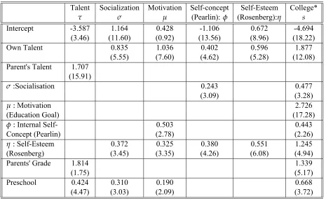
We estimated Logit models for the cognitive and non-cognitive skills for the child sample. These parameter estimates are then used to fix the transition probabilityp(x′_{|x, a).}

We report in table 1 the parameter estimates for specifications in which only the significant regressors (xanda).In our structural maximum likelihood estimations, however, we have

reported sensitivity of parameter estimates for this specification and speciations in which we have used both significant and insignificant parameter estimates forp(x′|x, a).

From table 1, it is clear that after controlling for parents' grade, preschool experience has significantly positive effect on the socialization skill, the motivational skill and on the levels of talent and schooling but has no effect on Pearlin measure of internal self-cocept and the Rosenberg measure of self-esteem. The estimates in the table also show that level of talent has strong positive effect on all skills.

Table 1: Logit model of cognitive and non-cognitive skills.

Talent Socialization Motivation Self-concept Self-Esteem College*

τ σ µ (Pearlin): φ (Rosenberg):η s

Intercept -3.587 1.164 0.428 -1.106 0.672 -4.694

(3.46) (11.60) (0.92) (13.56) (8.96) (18.22)

Own Talent 0.835 1.036 0.402 0.596 1.877

(5.55) (7.60) (4.62) (5.28) (12.08)

Parent's Talent 1.707 (15.91)

σ:Socialisation 0.243 0.477

(3.09) (3.28)

µ:Motivation 2.726

(Education Goal) (17.28)

φ:Internal Self- 0.503 0.443

Concept (Pearlin) (2.78) (2.26)

η:Self-Esteem 0.372 0.325 0.380 0.551 1.245

(Rosenberg) (3.45) (3.35) (4.26) (6.08) (4.94)

Parents' Grade 1.814 1.339

(1.75) (5.17)

Preschool 0.424 0.310 0.190 0.668

(4.47) (3.03) (2.09) (3.72)

7.3

An Augmented Earnings Function - Role of cognitive and

non-cognitive skills

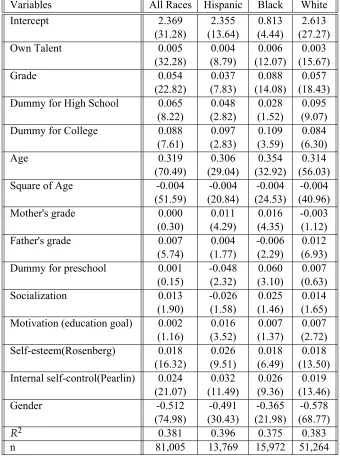
In this section we examine the effect on earnings of non-cognitive skills such as social, moti-vational, self-esteem and internal self-concept skills together with the effect of the cognitive skills such as innate ability and grades. The previous studies included only innate ability, schooling level and school quality as the main determinants of earnings. While preschool investment is an important determinant of these skills, we also included preschool binary variable as one of the regressors in the earnings function to see if it has an independent effect. In our specification, we included two dummy variables, High School (taking value 1 if a respondent had the high school degree) and College (if a respondent graduated from college). These dummy variables together with grade variable are to capture the earnings premiums for graduating from high school and college. Since we included AFQT score which is a reasonably good measure of one's innate ability, we do not have the ability biases in our estimates. We use the yearly earnings data to estimate the model.

Table 1 shows the parameter estimates of this augmented earnings function. The first column is for all three races together and the next three columns give the estimates for the Hispanics, Blacks and the Whites ethnic groups separately. It is clear from the estimates that after controlling for innate ability, family background and the schooling level, all four measures of non-cognititve skills have significant positive effect on earnings for all ethnic groups. Preschool has independent positive effect only for blacks. It is also interesting to note that a college graduate earns 8.35% higher returns in the overall population, and for Blacks and Hispanics this premium is even higher, slightly above 10%. The sociability skills are significant only for White but not for Black and Hispanic workers.

7.4

Estimation of Schooling Function

We consider two specifications of the schooling functions∗_(τ′_,σ′_,µ′_,η′_,φ′_{, a,ε}′_{). In the}

first specification, we assume that the schooling level is a continuous variable. We specify the optimal reaction functions∗_(τ′_,σ′_,µ′_,η′_,φ′_{, a,ε}′_{)as a linear function. We assume that}

the vector of random variableε′ constitutes the error term of the linear model and satisfies

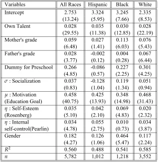
all the assumptions of the OLS model.2 _{We included the cognitive and non-cognitive skills} together with the family background variable as measured by the parent's education level. The parameter estimates from this model are shown in table 3 for all ethnic groups together,

2_{More generally we could assume thatE}(

Table 2: Determinants of earnings -- role of cognitive and non-cognitive skills (from the parent sample)

Variables All Races Hispanic Black White

Intercept 2.369 2.355 0.813 2.613

(31.28) (13.64) (4.44) (27.27)

Own Talent 0.005 0.004 0.006 0.003

(32.28) (8.79) (12.07) (15.67)

Grade 0.054 0.037 0.088 0.057

(22.82) (7.83) (14.08) (18.43) Dummy for High School 0.065 0.048 0.028 0.095

(8.22) (2.82) (1.52) (9.07) Dummy for College 0.088 0.097 0.109 0.084 (7.61) (2.83) (3.59) (6.30)

Age 0.319 0.306 0.354 0.314

(70.49) (29.04) (32.92) (56.03) Square of Age -0.004 -0.004 -0.004 -0.004

(51.59) (20.84) (24.53) (40.96) Mother's grade 0.000 0.011 0.016 -0.003

(0.30) (4.29) (4.35) (1.12) Father's grade 0.007 0.004 -0.006 0.012 (5.74) (1.77) (2.29) (6.93) Dummy for preschool 0.001 -0.048 0.060 0.007 (0.15) (2.32) (3.10) (0.63)

Socialization 0.013 -0.026 0.025 0.014

(1.90) (1.58) (1.46) (1.65) Motivation (education goal) 0.002 0.016 0.007 0.007 (1.16) (3.52) (1.37) (2.72) Self-esteem(Rosenberg) 0.018 0.026 0.018 0.018 (16.32) (9.51) (6.49) (13.50) Internal self-control(Pearlin) 0.024 0.032 0.026 0.019

(21.07) (11.49) (9.36) (13.46)

Gender -0.512 -0.491 -0.365 -0.578

(74.98) (30.43) (21.98) (68.77)

R2 _{0.381 0.396 0.375 0.383}

n 81,005 13,769 15,972 51,264

and also separately for the Hispanic, Black and White populations. It is clear from the estimates that the main determinant of grade is the innate ability measured by AFQT score. After controlling for family background, we find that the sociability skill has no effect on the schooling level.

In our second specification, we consider only two levels of schooling: college and more (s = 1), and no college (s = 0). Again we assume thats∗_(τ′_,σ′_,µ′_,η′_,φ′_{, a,ε}′_)is

repre-sented by a Probit model. We use a subset of the above regressors in this specification and use these estimates to calibrate our basic model in Eq. 2. The college status of parents is de-fined by assigning the value 1 if at least one parent had some college, and 0 otherwise. The parameter estimates from this model are shown in table 1 for all ethnic groups together. It is clear from the estimates that the main determinant of grade is again the innate ability mea-sured by AFQT score. After controlling for family background, we find that all cognitive and non-cognitive skills are significant determinants of the schooling level, the measure of motivational skills has the most significant positive effect on the probability of completing college.

7.5

Optimal Parental Preschool Investment Decision

We assume that the state variabless,τ,σ,µ,ηandφare all binary, all components of the

random vectorε is continuous which are observed by the decision maker but not by the

econometrician, and the preschool investment decision ais also a binary variable, taking value 1 when parents decide to invest in preschool and 0 otherwise. For most children, we have two parents but in our model we have assumed one parent. We could take mother as the parent. We have instead used both parent's information as follows: We construct parent's binary schooling variablesby assignings=1if the average grades of two parents

is more than12, otherwises = 0. We assume thatτis biologically inherited and it is not

influenced by preschool investment. We create the binary variableτassigning value1, i.e.,

an individual is highly talented if the AFQT score of the individual is70 or higher, and assigning value0otherwise.

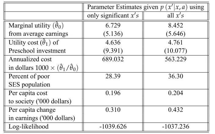
The estimate of the preschool investment cost depends on the calibrated value of the altruism parameterβas can be seen from table 5. Schweinhart et al. took average yearly

preschool cost to be $6178 per year. Consistent with their study, we calibrate the altruism parameter toβ=0.35for our analysis to be consistent with their cost estimate. The optimal

Table 3: Determinants of grade -- role of cognitive and non-cognitive skills (from the parent sample)

Variables All Races Hispanic Black White

Intercept 2.753 3.324 3.245 2.335

(13.24) (5.95) (7.66) (8.53)

Own Talent 0.028 0.035 0.030 0.028

(29.55) (11.38) (12.85) (22.19) Mother's grade 0.059 0.027 0.113 0.076

(6.48) (1.41) (6.03) (5.43) Father's grade 0.028 -0.002 0.004 0.067 (3.77) (0.12) (0.28) (6.44) Dummy for Preschool 0.266 -0.086 0.227 0.301 (4.85) (0.57) (2.25) (4.25)

σ:Socialization 0.037 -0.128 0.119 0.051

(0.83) (1.04) (1.34) (0.94)

µ:Motivation 0.458 0.425 0.348 0.468

(Education Goal) (40.75) (13.93) (14.98) (31.43)

η:Self-Esteem 0.035 0.042 0.069 0.020

(Rosenberg) (5.10) (2.10) (4.83) (2.32)

η:Internal 0.034 0.055 0.010 0.034

self-control(Pearlin) (4.78) (2.75) (0.73) (3.87)

Gender 0.182 0.126 0.464 0.117

(4.27) (1.06) (5.47) (2.24)

R2 _{0.560 0.488 0.541 0.585}

We consider a public policy of providing preschool to children of poor socioeconomic status (SES) in all periods. We define a parent to fall in the poor SES if his earnings is less than70percent of the average earnings in economy. This will incur a per capita cost, but such policy may also improve social mobility, earnings inequality and lead to a higher level of per capita long-run earnings. We examine if the gain from per capita earnings can outpace the cost of providing such a social insurance program. We also look at its within generation effects on earnings, and on intergenerational social and college mobility.

Table 4: Maximum likelihood parameter estimates given two different estimates of p(x′|x, a)and altruism parameterβ=0.35.

Parameter Estimates givenp(x′|x, a)using

only significantx′_{s allx}′_s

Marginal utility(θˆ₀) 6.729 8.452

from average earnings (5.136) (5.646) Utility cost (θˆ₁)of 4.636 4.761

Preschool investment (9.391) (10.077)

Annualized cost 689.032 563.229

in dollars1000×(θˆ₁/ˆθ₀)

Percent of poor 28.39 36.30

SES population

Per capita cost 0.196 0.204

to society ('000 dollars)

Per capita change 0.310 0.432

in earnings ('000 dollars)

Log-likelihood -1039.626 -1037.236

Note: Absolute value of t-statistics are in parentheses.

8

Economic Benefits from Public Provision of Preschool

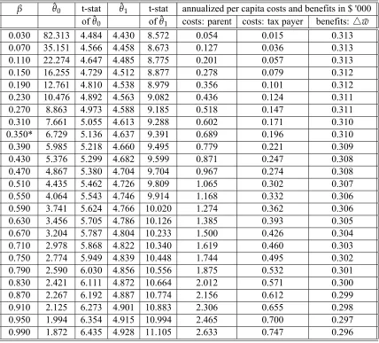
Table 5: Sensitivity of maximum likelihood estimates with variations of the altruistic pa-rameterβ.

β θˆ₀ t-stat θˆ₁ t-stat annualized per capita costs and benefits in $ '000

ofθˆ₀ ofθˆ₁ costs: parent costs: tax payer benefits: △¯w

0.030 82.313 4.484 4.430 8.572 0.054 0.015 0.313 0.070 35.151 4.566 4.458 8.673 0.127 0.036 0.313 0.110 22.274 4.647 4.485 8.775 0.201 0.057 0.313 0.150 16.255 4.729 4.512 8.877 0.278 0.079 0.312 0.190 12.761 4.810 4.538 8.979 0.356 0.101 0.312 0.230 10.476 4.892 4.563 9.082 0.436 0.124 0.311

0.270 8.863 4.973 4.588 9.185 0.518 0.147 0.311

0.310 7.661 5.055 4.613 9.288 0.602 0.171 0.310

0.350* 6.729 5.136 4.637 9.391 0.689 0.196 0.310

0.390 5.985 5.218 4.660 9.495 0.779 0.221 0.309

0.430 5.376 5.299 4.682 9.599 0.871 0.247 0.308

0.470 4.867 5.380 4.704 9.704 0.967 0.274 0.308

0.510 4.435 5.462 4.726 9.809 1.065 0.302 0.307

0.550 4.064 5.543 4.746 9.914 1.168 0.332 0.306

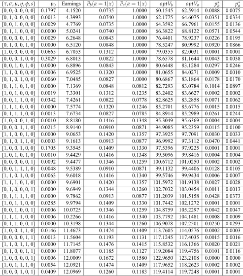
Table 6: Equilibrium Solution

[τ,σ,µ,η,φ, s] p0 Earnings Pb(a=1|x) Pa(a=1|x) optVb optVa p∗_b p∗a

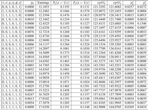
Table 7: Continuation of Table 6.

[τ,σ,µ,η,φ, s] p₀ Earnings P_b(a=1|x) Pa(a=1|x) optVb optVa p∗_b p∗a

preschool will depend on if the social protection will be available to all future generations or it is just a one time policy.

While looking at the magnitude of the estimated economic benefits below, it is important to keep in mind that the effects that we report are underestimated for many reasons: First, we have treated the Head Start children same as children without preschool. Second, the preschool programs that the respondents attended were the ones that existed during the six-ties. The quality of preschool programs ever since has improved significantly and thus the effects of current preschool programs will be much higher than the estimates that we have. Third, we have calibrated our model cost to a higher cost of a high quality pilot porgram.

Note that sinceεdoes not affect earnings, the optimaladepends only on the observable

component x of a parent's state variable, i.e. optimal preschool plan isa(x). In the

ab-sence of the social contract, suppose the parents follow the optimum preschool investment plansa(x)as shown in table 6. The invariant distribution of the corresponding transition

matrix{p(x′|x, a(x)), x∈ X}is shown in table 6 under the heading P_b(a=1|x). The

interpretation of this invariant distribution is as follows: IfPb(a=1|x)is the distribution

of population over the observable states of generationt, and the parents of generationt fol-low the optimal preschool investment plana(x), the distribution of population of the next

generation will also beP_b(a=1|x).

8.1

Social Mobility

A number of mobility measures for a transition matrix appear in the literature. Sommers and Conlisk (1979) argued that out of the existing measures,1−λ_maxis the most appropriate

measure of social mobility, where λ_max is the second highest positive eigenvalue of the

transition matrix (the highest positive eigenvalue of a transition matrix is always 1). We use this measure of social mobility to examine how the introduction of the social contract would improve social mobility. Our estimate of the measure of social mobility before the introduction of the social contract is0.568759and after the introduction of the social contract program, it improves to0.598074. The estimate of0.568759for the measure is very close to the estimates found in other studies of social mobility in the US.

8.2

College Mobility

Denote byQs ₌ [

qij], i, j = 1, 2, the intergenerational college mobility matrix in which

state 1 represents no college and state 2 represents college and higher. The element qij

to the college education status j, for all iand j = 1, 2. We report below the estimated

college mobility matrices, the corresponding invariant distributions, and the estimates of the mobility measure before and after the introduction of the social contract. These estimates indicate that the introduction of the social contract will increase college enrollment from a32.90percent to a 37.21percent, i.e. a4.31percent increase for a child of non-college parent. And the percentage of college enrolled population will increase in the long-run from the rate of48.17percent without social contract to a higher rate of51.18percent with the social contract. That is, there will be about a3.01% increase in college enrollments in the long-run.

College mobility statistics before introduction of social contract:

Qs_b=

[

0.6710 0.3290 0.3541 0.6459

]

, ps_b=[

0.518327 0.481673 ]

, 1−λs_max,b =0.683070

College mobility statistics after introduction of social contract:

Qs a =

[

0.6279 0.3721 0.3550 0.6450

]

, ps

a =[ 0.488177 0.511823 ], 1−λsmax,a =0.727102

8.3

Income Inequality

Preschool experience will increase the incomes of the children of poor SES and thus it will reduce the income gap between the rich and the poor. Using the Gini-coefficient to measure income inequality, we would expect that over time the income inequality will improve. In the long-run, the income distribution that one observes is the invariant distribution. Thus we compute the Gini-coefficient of income inequality for the invariant income distribution before the introduction of the social contract and compare it with the Gini-coefficient for the invariant income distribution after the introduction of the social contract. The estimated Gini-coefficients are respectively0.2133without the social contract, and 0.2087with the social contract. The estimated Gini-coefficient of earnings0.2133turns out to be very close to the estimates found in other studies on US. We note that the social contract of publicly providing preschool to children of poor SES leads to a significant reduction in the inequality of the long-term earnings.

8.4

Tax Burden of the Social Contract

the resource needs of the program will become smaller, and the tax revenues will become higher over time. We can look at the stream of these costs and benefits to the society and then compute the average per period costs and benefits to calculate the tax-burdens of the social contract. Applying the Ergodic theorem, however, this boils down to computing the costs and benefits of the invariant distribution that will result after the introduction of the social contract.

Approximately28.39percent of the population will fall in the poor socioeconomic status using our definition. Thus the per capita cost of the social contract to the economy in the long-run is$195.638but the gain in per capita income due to the introduction of the social contract is $309.60, so there is a net gain to the economy. This net gain is based on a reasonable value of the altruistic parameter β. The simulation results in our sensitivity

analysis shows that, the lower is the value of the altruism parameterβ,the higher is the gain

from the introduction of the social contract. The economic reason for this is quite obvious. When parents have lower altruism towards children, they will invest less on their children's preschool since such investment decreases their own felicity index and increase welfare of the children which got a lower weight whenβhas lower value. This estimate of net gain is

based on calibrating the value of βto the cost data of a high cost program as noted earlier

whose benefits are supposed to be higher than our estimated benefits. Thus, this gain is an underestimate of the actual net benefit. Furthermore, our benefit calculation does not take into account other public savings such as savings from welfare assistance programs and savings to the criminal justice system and potential victims of crimes. If we incorporate these, the returns will be much higher. Using data from the High/Scope Perry Preschool Program, Schweinhart et al. estimated a total benefit of $7.16 from all these sources for each dollar spent on the preschool program.

9

Conclusion

This paper formulated an altruistic model of parental preschool investment within a struc-tural dynamic programming framework. The paper provided conditions for the local and global identification of the non-parameteric and parametric structural parameters of the dy-namic programming model. It used the NLSY79 and NLSY79 Children and Young Adult datasets for all emprical estimations of the model.

the motivational skill, the Rosenberg measure of self-esteem skill and the Pearlin mastery scale of internal self-concept skill. The paper found that the preschool boosted significantly all the cognitive and non-cognitive skills, but not the Rosenberg measure of self-esteem skill and the Pearlin measure of internal self-concept skill. Moreover, all these cognitive and non-cognitive skills have significant positive effects on the level of schooling and the labor market earnings of individuals.

The paper estimated the structural parameters and then used those to carry out a Lucas-Critique free policy analysis to examine the effect of publicly providing preschool to eco-nomically disadvantged children. Taking into account the within generation and between in-tergenerations effects of such a policy, the paper estimates that in the long run the preschool social contract policy

• improves the social mobility from0.569to0.598,measured in a scale of0to1.

• improves the college mobility from0.683to0.727,measured in a scale of0to1and increases the college completion rate of the children of non-college educated parents from32.9percent to37.21percent, i.e., a4.31percent increase.

• reduces the earnings inequality measured by the Gini coefficient in a scale of0to1 from0.213to0.209.

The paper estimates that the preschool social contract policy costs the economy $195.64 per capita but increases the per capita earnings by $309.60. That is, there is a significant net positive gain to the tax payers from the introduction of the preschool social contract program.

References

Aguirregabiria, V. and P. Mira (2002), "Swapping the Nested fixed Point Algorithm: A Class of Estimators for Discrete Markov Decisions Models,"Econometrica, vol.70(4):1519-1543.

Barnett, W. Steven (1995), “ Long-Term Effects of Early Childhood Programs on Cogni-tive and School Outcomes,”The Future of Children: Long-Term Outcomes of Early Childhood Programs, Vol. 5(3):25-50.

Bhattacharya, R. and M. Majumdar (1989), "Controlled Semi-Markov Model -The Dis-counted Case,"Journal of Statistical Planning and Inference, vol.21:365-381. Campbell, F. A., R. Helms, J.J. Sparling and C. T. Ramey (1998) “Early Childhood

Pro-grmas and Success in School: The Abecedarian Study” in (eds) W. Steven Barnett and Sarane Spence Boocock, “Early Care and Education for Children in Poverty: Promises, Programs, and Long-Term Results”, State University of New York Press, New York.

Coleman James et al. (1966), “Equality of Educational Opportunity,” Washington DC, U.S. GPO.

Cunha, Flavio, James J. Heckman, Lancel Lochner and Dimitry V. Masterov (2006), "In-terpreting the evidence of life cycle skill formaiton," Chapter 12, in (eds) Eric A. Hanushek and Finis Wetch, "Handbook of the Economics of Education," Volume 1, Elsevier B.V.

Currie, Janet (2001) "Early Childhood Education Programs," Journal of Economic Per-spectives,vol.15(2):213-238.

Currie, Janet and Duncan Thomas(2000), "School Quality and Longer Term Effect of Head Start,"Journal of Human Resources, Vol. 35(4):755-74.

Currie, Janet and Duncan Thomas(1995), "Does Head Start Make a Difference?," Ameri-can Economic Review, Vol. 85, No. 3., pp. 341-364.

Entwisle, Dorris (1995) ”The Role of Schools in Sustaining Early Childhood Program Ben-efits,”The Future of Children: Long-Term Outcomes of Early Childhood Programs, Vol. 5(3).

Hansen Lars Peter and Thomas Sargent (1981), "Formulating and Estimating Dynamic Linear Rational Expectations Models," in Lucas, Robert and Thomas Sargent (eds), "Rational Expectations and Econometric Practice": Minneapo1is:University of Min-nesota Press.

Hanushek, Eric A. (1986), “The Economics of Schooling: Production and Efficiency in Public Schools,”Journal of Economic Literature,Vol. 24, No. 3. pp. 1141-1177. Heckman, James (2000) "Policies to Foster Human Capital,"Research in Economics,

54(1):3-56.

Hotz, J. and R. A. Miller (1993), "conditional Choice Probabilities and the Estimation of Dynamic Models,"Review of Economic Studies, Vol.60:497-529.

McCormick, Kathleen (1989), “An Equal Chance: Educating At-Risk Children to Suc-ceed,” Alexandria, Virginia: National School Board Associations.

McFadden, Daniel (1981), "Econometric Models of Probabilistic Choice," in (eds), C. Manski and D. McFaden "Structural Analysis of Discrete Data with Econometric Ap-plications," Cambridge, MA: MIT Press.

Mohanty, Lisa and Lakshmi K. Raut (2009), "Home Ownership and School Outcomes of Children: Evidence from the PSID Child Development Supplement,"American Journal of Economics and Sociology,68:2, 465-489.

Nishimura, Kazuo and Lakshmi K. Raut (2007), "School Choice and the Intergenerational Poverty Trap,"Review of Development Economics,11(2) , 412-420,2007.

Pearlin, Leonard I.; Lieberman, Morton A.; Menaghan, Elizabeth G.; and Mullan, Joseph T. (1981), "The Stress Process,"Journal of Health and Social Behavior22 (Decem-ber): 337-353.

Praskash Rao, B. L. S. (1992), "Identifiability in Stochastic Models: Characterization of Probability Distributions," New York: Academic Press, Inc.

Raut, Lakshmi K. (1995), “Signaling Equilibrium, Intergenerational Social Mobility and Long Run Growth,” draft presented at the Seventh World Congress Meeting of the Econometric Society, Tokyo, 1995 http://papers.ssrn.com/abstract=852924.

Rosenberg, Morris. (1965), "Society and the Adolescent Self- Image. Princeton," New Jersey: Princeton University Press.

Rust, John (1987), "Optimal Replacement of GMC Bus Engines: An Empirical Model of Harold Zurcher,"Econometrica,Vol. 55(5),999-1033.

Rust, John (1994), “Structural Estimation of Markov Decision Processes”, in (eds) R.F. Engle and D.L. MacFadden, “Handbook of Econometrics, Volume IV,” Elsevier Sci-ence B.V.

Schweinhart, Lawrence J., Helen V. Barnes, and David P. Weikart (1993) “Significant Ben-efits: The High/Scope Perry Preschool Study Through Age 27,” Ypsilanti, Michigan: The High/Scope Press.

Sommers, Paul. M. and John Conlisk (1979), “Eigenvalue Immobility Measures for Markov Chains”,Journal of Mathematical Sociology, vol.6:253-276.