A Multivariate Generalized Orthogonal Factor GARCH Model

Munich Personal RePEc Archive

A Multivariate Generalized Orthogonal

Factor GARCH Model

Lanne, Markku and Saikkonen, Pentti

University of Helsinki, HECER

May 2005

Online at

https://mpra.ub.uni-muenchen.de/23714/

öMmföäflsäafaäsflassflassflas ffffffffffffffffffffffffffffffffffff

Discussion Papers

A Multivariate Generalized Orthogonal Factor

GARCH Model

Markku Lanne

University of Jyväskylä, RUESG and HECER

and

Pentti Saikkonen

University of Helsinki, RUESG and HECER

Discussion Paper No. 63 May 2005

ISSN 1795-0562

HECER

Discussion Paper No. 63

A Multivariate Generalized Orthogonal Factor

GARCH Model*

Abstract

The paper studies a factor GARCH model and develops test procedures which can be used to test the number of factors needed to model the conditional heteroskedasticity in the considered time series vector. Assuming normally distributed errors the parameters of the model can be straightforwardly estimated by the method of maximum likelihood. Inefficient but computationally simple preliminary estimates are first obtained and used as initial values to maximize the likelihood function. Maximum likelihood estimation with nonnormal errors is also straightforward. Motivated by the empirical application of the paper a mixture of normal distributions is considered. An interesting feature of the implied factor GARCH model is that some parameters of the conditional covariance matrix which are not identifiable in the case of normal errors become identifiable when the mixture distribution is used. As an empirical example we consider a system of four exchange rate return series.

JEL Classification: C32, C51, F31.

Keywords: Multivariate GARCH model, mixture of normal distributions, exchange rate.

Markku Lanne Pentti Saikkonen

University of Jyväskylä University of Helsinki School of Business and Economics Department of Statistics P.O. Box 35 (MaE) P.O. Box 17 (Arkadiankatu 7) FIN-40014 University of Jyväskylä FI-00014 University of Helsinki

FINLAND FINLAND

e-mail:[email protected] e-mail:[email protected]

1 Introduction

Even though the literature on volatility models is huge, only a relatively small

frac-tion of it is devoted to developing and applying multivariate GARCH models. This

is not due to the lack of interest or importance because understanding the

comove-ments of financial returns is at the heart of empirical finance and models capable of describing the joint behavior of asset prices are in great demand in areas such as asset

allocation and risk management. It is rather the practical problems inherent in most

multivariate GARCH models that have retarded their widespread use. The problems

with estimation are mainly caused by the typically quite rapid increase in the number

of parameters with the dimension of the system and the restrictions required by the

positive definiteness of the conditional covariance matrix. As one solution to these problems, several factor and orthogonal models have been introduced in the literature.

Factor models assume the data to be generated by a set of uncorrelated

compo-nents and in orthogonal models these compocompo-nents are also (a subset of) the principal

components of the data. According to the taxonomy of Bauwens et al. _{(2003), in}

orthogonal models the matrix by which the data are obtained from the components

must be orthogonal, while in generalized orthogonal models its invertibility suffices.

The notion of a factor model typically encompasses the idea that there are a relatively

small number of common underlying variables, whereas (generalized) orthogonal

mod-els (e.g. van der Weide, 2002, Vrontos et al._{, 2003) commonly do not have a reduced}

number of principal components. Thus, (generalized) orthogonal models are rather

restrictive for financial data in that they allow for no idiosyncratic shocks.1

In this paper we introduce a new kind of generalized orthogonal GARCH model

that allows for a reduced number of conditionally heteroskedastic factors and, hence,

idiosyncratic shocks. Therefore we call our model a generalized orthogonal factor

1_{Orthogonal models with fewer principal components than time series have also been presented}

(see e.g. Alexander, 2001), but they are hampered by the fact that the conditional covariance matrix

GARCH model. Our model is related to the factor GARCH model of Engle et al.

(1990), but it is more parsimonious and easier to estimate. Gaussian maximum

likeli-hood (ML) estimates can be straightforwardly obtained and likelilikeli-hood functions based

on other distributions, such as the (multivariate) t distribution, can also be readily

formulated. This is illustrated by the empirical application of the paper where,

in-stead of the commonly used t distribution, a mixture of normal distributions is more

appropriate and, therefore, applied. Interestingly, some parameters of the conditional

covariance matrix, which are not identifiable in the Gaussian model, become identifi -able in a model based on a mixture of normal distributions. In practice thefirst step of applying any factor GARCH model consists of selecting the unknown number of

conditionally heteroskedastic common factors. In order to facilitate this selection two

tests are developed in the paper.

The remainder of the paper is organized as follows. The model is introduced in

Section 2. Parameter estimation and statistical inference are discussed in Section 3

assumingfirst a Gaussian likelihood and providing thereafter an extension to the case of a mixture of normal distributions. Section 4 develops tests for checking the number

of conditionally heteroskedastic common factors. Section 5 presents an application to

a data set of exchange rate return series. Finally, Section 6 concludes.

2 Model

Consider ann-dimensional time seriesyt (t= 1,2, ...) generated by

yt =W Ht1/2εt, (1)

whereW (n×n)is a nonsingular parameter matrix, Ht (n×n) is a stochastic (a.s.) positive definite diagonal matrix measurable with respect to the information set

Ft−1 = {yt−j, j ≥1}, and εt (n×1) is a sequence of independent and identically distributed random vectors with zero mean and identity covariance matrix or, briefly,

difference sequence and, givenFt−1, the conditional covariance matrix of yt is

Covt₋1(yt) = W HtW0 def

= Σt. (2)

Equations (1) and (2) specify a general model for conditional heteroskedasticity of the

time series vectoryt.To make this general model feasible in practice, the dependence of the diagonal elements of the matrixHt on past values of yt has to be specified.

A model similar to that defined by equations (1) and (2) has recently been con-sidered by van der Weide (2002) and Vrontos et al. _{(2003) (see also Klaassen (2000)}

and Alexander (2001)). These authors do not explicitly discuss the case where some

of the diagonal elements of the matrix Ht are constant, that is, independent of t. Because we feel that it is of interest to allow for this possibility we shall assume that

Ht =diag[Vt :In−r], (3)

whereVt=diag[v1t · · · vrt]and0≤r≤n. Thus, we have to specify the dependence of vit (i= 1, ..., r) on past values of yt. Unless otherwise stated, it will henceforth be assumed that r > 0 so that the quantities v1t, ..., vrt are all stochastic, and hence, time varying. In order to motivate the employed specification, write W = [W1 :W2]

and W−1 _{= B}0 _{= [B}

1 :B2]0 where the matrices W1 and W2 are of orders n×r and

n×(n₋r),respectively, and the matrixB0_{is partitioned conformably. From equation} (1) one then obtains

B0

1yt =Vt1/2ε1t (4) and

B₂0yt=ε2t, (5)

where εt = [ε01t ε02t] 0

is partitioned in an obvious way. Thus, the components of B0

1yt are uncorrelated univariate conditionally heteroskedastic processes whereas B0

2yt ∼ i.i.d.(0, In−r). As in van der Weide (2002) and Vrontos et al. (2003) we specify the diagonal elements ofVtas standard GARCH processes driven by squared lagged values of the components ofB0

1yt. For ease of exposition, we assume the GARCH(1,1) models

where b0

1i signifies the ith row of the matrix B10 and the other parameters satisfy

αi >0, βi ≥ 0 and βi +αi < 1 for all i = 1, ..., r. The inequality αi > 0 is due the assumption that vit does not reduce to constant.

The imposed parameter restrictions imply that, under mild conditions about the

density of εt, the vector process yt defined by equations (1), (3) and (6) is strictly stationary and ergodic and also second order stationary (see Engle and Kroner (1995)

and Comte and Lieberman (2003)). Note also that the intercept terms in (6) are

nor-malized in such a way that the components ofB0

1ythave unit unconditional variance. These normalizations will be convenient in our subsequent developments. Combined

with the assumption that the variances of the components of ε1t are normalized to unity they ensure that the parameters in equations (4) and (6) are unique up to

multiplying the columns ofB1 by minus one.

Because equation (5) can be premultiplied by any orthogonal (n−r)×(n−r)

matrix without changing the second order properties of the model the parameter

matrixB2 is not identifiable without further assumptions. The special casen−r= 1

is an exception in that identifiability obtains up to multiplying (the vector) B2 by

minus one. Similar conclusions, of course, hold for the parameter matrix W2. In this

section we shall only rely on second order properties of the series yt and, therefore, identifiability of the parameter matrices B2 and W2 is not achieved. This means, in

particular, that part of the subsequent discussion is only relevant when the error term

εtis normally distributed or, more generally, has a spherically symmetric distribution such as a t distribution.2 _{However, it will be seen later that with other distributions}

even the parameter matrices B2 and W2 may become identifiable (up to multiplying

the columns by minus one).

As in van der Weide (2002), we factorize the parameter matrix W but, instead of 2_{The distribution of a random vector x is spherically symmetric if x and Ox have the same}

the singular value decomposition used in that paper, we use the polar decomposition

W =CR, (7)

whereC(n×n)is a (symmetric) positive definite matrix andR(n×n)is an orthog-onal matrix. The nonsingularity of the matrix W ensures the positive definiteness of the matrix C and uniqueness of the decomposition (see Horn and Johnson (1985), p. 413). The normalizations used in (6) imply that E(Vt) =In−r.Thus, it follows from equations (2) and (3) that the covariance matrix ofyt satisfies

Cov(yt) def

= Ω=W W0 =CC0. (8)

Let Ω=PΛP0 _{be the spectral decomposition of the covariance matrix Ωso that}

Λ is a diagonal matrix containing the eigenvalues of Ω on the diagonal and P is an orthogonal matrix of corresponding eigenvectors. Thus, the matrix C is the unique (positive definite) square root of the covariance matrix Ω, that is, C = PΛ1/2_P0 ₌

Ω1/2_{, whereas R = Ω}−1/2_{W. Because the theoretical covariance matrix Ω can be}

consistently estimated by the sample covariance matrix the continuity of the mapping

Ω _→ Ω1/2 _{implies that the matrix C can be consistently estimated by using the}

spectral decomposition of the sample covariance matrix. Part of the parameter matrix

W can therefore be consistently estimated in a very simple way.

The polar decomposition assumed in (7) is not the only possibility one could

entertain. As already mentioned, van der Weide (2002) used the singular value

de-composition and defined the matrix C as C =PΛ1/2 _{with P andΛ as above. Unlike}

the polar decomposition, this factorization is unique only when the eigenvalues of Ω

are distinct. Uniqueness is a useful property if the components of the factorization

are estimated simultaneously. Instead of the polar decomposition, uniqueness can be

achieved by an appropriate version of the QR decomposition (see Horn and Johnson

(1985), p. 112-114). In what follows, the QR decomposition can be used instead of

In the model of Vrontos et al. _{(2003) the parameter matrix W is assumed to}

be lower triangular. This is a simplifying assumption which is not without loss of

generality because, in general, the orthogonal matrix R cannot be dropped from (7) and because the application of the Cholesky decomposition to the conditional

covari-ance matrixΣt does generally not imply a factorization of the form (2) withW lower triangular.3 _{In addition to being restrictive, the lower triangularity assumption of the}

matrix W involves the difficulty that a certain order is assumed for the components

of the vector yt.

By the above discussion we can write equation (1) as

yt=W1Vt1/2ε1t+W2ε2t. (9)

This means that the model can be interpreted as a factor GARCH model in which

the conditional heteroskedasticity is due to r common factors, the components of the vector Vt1/2ε1t. Alternatively, the model implies the existence of n− r linearly independent homoskedastic linear combinations of the process yt given by equation (5). Now, partition R = [R1 :R2] conformably with the partition of W so that

W1 =CR1 and W2 =CR2. Using equation (8) and the fact that R1R01+R2R02 =In it is easy to check that the conditional covariance matrix (2) can be written as

Σt=Ω+CR1(Vt−Ir)R01C0 (10)

or, alternatively, as

Σt =Ω∗+ r

X

i=1

vitw1iw10i, (11)

where Ω∗ _=W

2W20 andw1i signifies the ith column of the matrixW1.

Equation (11) shows that in our model the conditional covariance matrix is similar

to that in the factor GARCH model of Engle et al. (1990). A major difference

between the conditional covariance matrices arising from these two models lies in their

3_{A multivariate GARCH model based on the Cholesky decomposition of the conditional}

constant terms. In our model the constant term is closely related to the unconditional

covariance matrix Ω whereas in the model of Engle et al. _{(1990) the constant term}

has no particular role. Note also that in the representation (11) the constant term

Ω∗ _{is singular and its rank is directly related to the number of common factors. In}

the model of Engle et al. _{(1990) the corresponding constant term is assumed to be}

positive semidefinite and it has typically been treated as a positive definite matrix. This implies that our model is generally more parsimonious than the model of Engle

et al. (1990). Another difference between the two models concerns the correlation

of the common factors. As typical in factor models, our model assumes uncorrelated

common factors whereas in the model of Engle et al. _{(1990) the common factors}

are generally correlated although their conditional covariance is constant. These

differences have important implications on the estimation of the parameters of the

model. Above we already discussed the (preliminary) estimation of the covariance

matrix Ω by using its sample analog and in the next section it will be seen that

convenient (preliminary) estimators can also be obtained for other parameters of our

model. Finally, note that Engle et al. _{(1990) list some attractive properties of the}

conditional covariance structure implied by their model. These properties, which

include the positive (semi)definiteness of the conditional covariance matrix, are also shared by the conditional covariance matrix arising from our model.

As with the factor GARCH model of Engle et al. _{(1990), our model can also be}

viewed as a special case of the BEKK model of Engle and Kroner (1995). Specifically, note that from equations (2) and (3) it follows thatvit =b01iΣtb1i which in conjunction with equations (6) and (11) yields

Σt=Ω∗∗+ r

X

i=1

(β_ib0_1iΣt−1b1i+αib01iyt−1yt−1b1i)w1iw01i,

where Ω∗∗ = Ω∗ +Pr_i=1(1−αi−βi)w1iw01i. This shows the aforementioned connec-tion with the BEKK model. An implicaconnec-tion of this is that the asymptotic estimaconnec-tion

results obtained by Comte and Lieberman (2003) for Gaussian ML estimators in the

3 Parameter Estimation

3.1 Gaussian ML Estimation

The parameters of the model introduced in the previous section can be estimated by

Gaussian ML. Thus, assume that, conditional onFt−1,the distribution ofytis normal with zero mean and covariance matrix Σt. The related conditional density is

ft−1(yt) = (2π)−n/2det (Σt)−1/2exp

½

−1

2y

0 tΣ−t1yt

¾

.

From equations (2), (3) and (8) it follows that det (Σt) = det (Ω)v1t· · ·vrt and

y0

tΣ−t1yt = yt0BHt−1B0yt = y0tB1Vt−1B10yt+y0tB2B20yt where Bi = C−10Ri (i = 1,2) by equation (7). Thus, because R1R01 +R2R20 = In and Ω = CC0, we can write

y0

tΣ−t1yt=y0tC−10R1(Vt−1 −Ir)R01C−1yt+yt0Ω−1yt and, furthermore,

ft−1(yt) = (2π)−n/2det (Ω)−1/2exp

½

−1₂y0_tΩ−1yt

¾

(12)

×

r

Y

i=1

v_it−1/2exp

½

−1

2y

0

tC−10R1(Vt−1−Ir)R10C−1yt

¾

.

Equation (6) shows that, in addition to the GARCH parametersαiandβi(i= 1, ..., r), the diagonal matrix Vt depends on the parameter matrix B1 or on C−10R1. Thus,

since Ω=CC0_{, the Gaussian likelihood depends on the parameters C, R}

1, αi andβi

(i= 1, ..., r).Instead ofC it appears to be convenient to use its inverse on which the likelihood function only depends.

Assume that we have an observed data set y0, ..., yT. The first observation y0 is

used as an initial value in the GARCH models (6) and the subsequent analysis will

be conditional on it and also onvi0 (i= 1, ..., r).Letρ1i signify theith column of the matrixR1and setΦ=C−1 andδ = [δ01 · · · δ

0 r]

0

whereδi = [αi βi] 0

(i= 1, ..., r).From the expression of the conditional density function (12) and the subsequent discussion

can be written as

lT (Φ, R1, δ) =T log det (Φ)− 1 2

T

X

t=1

y_t0Φ0Φyt (13)

− r

X

i=1

Ã

1 2

T

X

t=1

logvit+

1 2

T

X

t=1

(v−_it1−1)(ρ0_1iΦyt)2

!

def

= l0T (Φ) + r

X

i=1

liT(Φ, ρ1i, δi).

Here we have also made use of the fact that, in addition to the parameter δi, the conditional variance vit only depends on the parameters ρ1i andΦ (see equation (6) and note that b0

1iyt−1 =ρ01iΦyt−1). We need to maximize lT (Φ, R1, δ) subject to the

constraints

ρ0_1iρ_1j =

  

1, i=j

0, i6=j . (14)

The required maximization is obviously a highly nonlinear problem. Good initial

values are therefore desirable for successful numerical optimization of the likelihood

function.

As discussed in the previous section, a consistent estimator of Ω can be obtained

from the (uncentered) sample covariance matrix

e

Ω=T−1

T

X

t=1

ytyt0.

A consistent estimator of the matrix Φ, denoted by Φe, can be obtained from Ωe.

The estimatorΦe can be either the (unique) square root ofΩe−1 _{or its Cholesky factor}

depending on which one of the two alternative specifications is adopted. Note that the estimatorΦe can be obtained by maximizing thefirst component of the log-likelihood function, that is,l0T (Φ). Although consistent, the estimatorΦe is therefore inefficient because it ignores the second component of the log-likelihood function which is due

to conditional heteroskedasticity (cf. van der Weide (2002)).

Obtaining initial estimates for the parameters R1 and δ is more complicated.

carried out separately fori= 1, ..., r.Define the set ∆1 ={(ρ11, δ1) :ρ011ρ11 = 1}and,

for i= 2, ..., r, ∆i =

©

(ρ_1i, δi) :ρ01iρ1i = 1, ρ01iρ1j = 0, 1≤j ≤i−1

ª

. Then consider estimators defined by

(_eρ₁₁,eδ1) = arg max (ρ₁₁,δ1)∈∆1

l1T(Φe, ρ11, δ1)

(15)

(_eρ_1i,eδi) = arg max

(ρ1i,δi)∈∆˜i

liT(Φe, ρ1i, δi), i= 2, ..., r,

where∆˜i is defined by replacingρ1j in the definition of∆i byeρ1j.It is straightforward to see that solving theserseparate maximization problems is equivalent to maximizing the functionlT(Φe, R1, δ)subject to the constraints (14). Thus, because the estimator

e

Φ is consistent the consistency of the estimators Re and eδ formed from _eρ_1i and eδi

(i= 1, ..., r) is expected to hold under appropriate regularity conditions.

Once the initial estimators Φe, Re and eδ are available one can use numerical op-timization methods to maximize the likelihood function lT (Φ, R1, δ) subject to the

constraints (14). This optimization yields Gaussian ML estimates for the parameters

Φ, R1 and δ denoted byΦb, Rb1 andbδ, respectively. Gaussian ML estimates of other

parameters can be formed from these estimates by transformations. For instance, the

Gaussian ML estimate of Ω is Ωb =Φb−1_Φb−10 _{and, sinceW}

1 =Φ−1R1 and B1 =Φ0R1,

the Gaussian ML estimates of W1 andB1 are Wc1 =Φb−1Rb1 andBb1 = Φb0Rb1,

respec-tively. One can also estimate the parameters W2 andB2 but first an estimate for R2

has to be obtained. For anyk×l matrix A of full column rank letA_⊥ be its orthog-onal complement, that is, any k×(l−k) matrix of full column rank and such that

A0_A

⊥ = 0. Then a Gaussian ML estimate of R2 is given by Rb2 = Rb1⊥(Rb01⊥Rb1⊥)−1/2

and Gaussian ML estimates of W2 and B2 are Wc2 = Φb−1Rb2 and Bb2 = Φb0Rb2,

respec-tively. These estimates are not unique (and hence not consistent) but they can be

used to provide unique (and consistent) estimates for some derived parameters. For

instance, Ωb∗ _{= cW}

2Wc20 is the unique Gaussian ML estimate of the parameter Ω∗ in

3.2 Limiting Distributions of Gaussian ML Estimators

Because our model is a special of the BEKK model asymptotic properties of the

Gaussian ML estimators Φb, Rb1 andbδ can be inferred from the results of Comte and

Lieberman (2003). Under regularity conditions these results hold even if the true

likelihood is not Gaussian.

Denote θ = £vec(R1)0 vech(Φ)0 δ01 · · · δ0r

¤0

and let bθ signify the corresponding vector of Gaussian ML estimators. Here vec and vech signify the usual vectorization

and half vectorization operators, respectively (see Chapter 7 in Lütkepohl (1996)).

The parameter vector θ satisfies the identifying constraints (14) which can be ex-pressed in matrix form as

g(θ)def= Lrvec(R0₁R1)₋vech(Ir) = 0.

HereLr is the 1₂r(r+ 1)×r2 elimination matrix defined by the equation vech(A) =

Lrvec(A) where A is an r×r matrix. We also introduce the r2_×r2 _commutation

matrix Krr defined by Krrvec(A) =vec(A0)with A as above. Then,

∂g(θ)/∂vec(R1)0 = [Lr(Ir2 +K_rr) (I_r⊗R0₁) : 0]

def

= G,

where ⊗denotes the Kronecker product (cf. result 10.5.1(2a) in Lütkepohl (1996)).

The limiting distribution of the estimatorbθ can be obtained by using Theorem 4 of Comte and Lieberman (2003) and well known results of constrained (quasi) ML

estimation based on the use of Lagrange multipliers. Note, however, that the usual

procedure described in Aitchison and Silvey (1958) and Davidson (2000, p. 289-290)

needs to be modified because the (Gaussian) information matrix is singular. This feature can be dealt with by using the modification described in Silvey (1959). To this end, let ¯lt(θ) signify the Gaussian log-likelihood of the tth observation, that is,

¯

lt(θ) = logft−1(yt) with ft−1(yt) defined in (12) and interpreted as a function of the parameter vector θ. The idea is to replace the information matrix of a single observation, that is, −E(∂2¯_l

t(θ)/∂θ∂θ0) byJ def

= G0_G−E(∂2¯_l

likelihood is not Gaussian but appropriate regularity conditions hold,

T1/2(bθ−θ)→d N(0, Q1Q0Q1), (16)

where Q0 = E

¡

(∂¯lt(θ)/∂θ)(∂¯lt(θ)/∂θ0)

¢

and Q1 = J−1 −J−1G0(GJ−1G0)− 1

GJ−1_.

In the case of Gaussian likelihood the limiting distribution simplifies because then

Q0 = J − G0G and, consequently, Q1Q0Q1 = Q1. A consistent estimator of the

matrix Q0 is given by Qb0 = T−1PT_t=1(∂¯lt(bθ)/∂θ)(∂¯lt(bθ)/∂θ0) and a consistent esti-mator of the matrix Q1 is obtained by replacing the matrices J and G in the de-finition of Q1 by consistent estimators. A consistent estimator of the matrix J is

b

J =Gb0_Gb−T−1PT

t=1Et−1(∂2l¯t(θ)/∂θ∂θ0)_|θ=bθ where Gb = [Lr(Ir2+Krr) (Ir⊗Rb 0

1) : 0]

is a consistent estimator of G. Here Et₋1(∂2¯_l

t(θ)/∂θ∂θ0)_|θ=bθ could be replaced by

∂2¯lt(bθ)/∂θ∂θ0 but, according to Hafner and Herwartz (2003), the given form is prefer-able. As advocated by these authors, we use analytical derivatives instead of numerical

ones to estimate the limiting covariance matrix in (16). Approximate standard errors

for the components of the estimator vectorbθ can be obtained by taking square roots of the diagonal elements of the matrixQb1Qb0Qb1.

From (16) it is straightforward to derive limiting distributions for other estimators

of which Wc1 and Bb1 are of special interest. Suppose the parameter matrix Φ is

symmetric. Then, it is straightforward to check that Wc1 −W1 = Φ−1(Rb1 −R1)−

Φ−1_(Φb−Φ)Φ−1_R 1+op

¡

T−1/2¢_{and, upon vectorizing and using the factΦ}−1_R

1 =W1,

one obtains

vec(Wc1)−vec(W1) = ¡Ir⊗Φ−1

¢ ³

vec(Rb1)−vec(R1)´

−¡W₁0 ⊗Φ−1¢Dn

³

vech(Φb)−vech(Φ)´+op

¡

T−1/2¢,

whereDn is then2×n(n+ 1)/2duplication matrix defined by vec(A) =Dnvech(A) for any symmetricn×nmatrix A. From this and (16) one obtains

T1/2³vec(Wc1)₋vec(W1)´_→d N(0, G2Q1Q0Q1G02), (17)

replacing the parameter matrices Φ and W1 in the definition of G2 by Φb and Wc1,

respectively. Here we assumed a symmetric specification for the parameter matrixΦ

and used the relation vec(Φ) = Dnvech(Φ). IfΦ is assumed lower triangular one can use a similar reasoning with the identity vec(Φ) =L0

nvech(Φ)(see result 9.6.3(1)(b) in Lütkepohl (1996)). Thus, in (17) and the subsequent discussion the matrixG2 should

be redefined by replacing the duplication matrix Dn by the transposed elimination matrix L0

n.

As for the estimatorBb1,we haveBb1−B1 =Φ0(Rb1−R1) + (Φb0−Φ0)R1+op¡T−1/2¢ from which it follows that

vec(Bb1)−vec(B1) = (Ir⊗Φ0)

³

vec(Rb1)−vec(R1)´ + (R0₁⊗In)

³

vec(Φb0)−vec(Φ0)´+op

¡

T−1/2¢.

Assume again first that the parameter matrix Φ is symmetric and note that then vec(Φ0_{) = K}

nnDnvech(Φ) and KnnDn = Dn (see results 7.2.3(a) and 9.2.3(2) in Lütkepohl (1996)). Hence, from the preceding equation and (16) we find that

T1/2³vec(Bb1)−vec(B1)

´ _d

→N(0, G3Q1Q0Q1G03), (18)

whereG3 = [(Ir⊗Φ0) : (R01⊗In)Dn : 0]and a consistent estimator of the covariance matrix of the limiting distribution is Gb3Qb1Qb0Qb1Gb03 with Gb3 defined in an obvious

way. If the parameter matrix Φ is assumed lower triangular we have vec(Φ0_{) =}

KnnL0nvech(Φ). Thus, (18) and the subsequent discussion apply with the duplication matrixDnreplaced byKnnL0n.Note that here, as well as in the corresponding previous cases, the product Qb1Qb0Qb1 can be replaced byQb1 if Gaussian likelihood is assumed.

In addition to approximate standard errors, the asymptotic results given in (16),

(17) and (18) can also be used to construct Wald tests for smooth constraints on the

involved parameters. It should be noted, however, that the limiting distributions in

(16), (17) and (18) are singular and therefore care is needed to make sure that the

conventional limit theory applies. For instance, in the case of the linear hypothesis

addition to this, the matrix A should be such that the matrix AG3Q1Q0Q1G03A0 is

positive definite.

The preceding estimation and testing results were based on Gaussian likelihood.

In the application of GARCH models it is frequently found that the normal

distrib-ution is not optimal and a more leptokurtic distribdistrib-ution, such as the t distribdistrib-ution,

should be used. It is not difficult to set up the likelihood function based on the t

distribution or any other spherical distribution and maximize it by numerical

meth-ods. For nonnormal distributions no factorization similar to that in (12) is possible,

however, and no formal proof of the asymptotic properties of the obtained estimators

and test statistics seems to be available.

Instead of distributions discussed above we shall consider a certain mixture of

normal distributions. This is motivated by our empirical applications where the t

distribution turned out to be inappropriate whereas a mixture distribution appeared

more reasonable.

3.3 ML Estimation Based on a Mixture of Normal Distributions

First suppose that the error term εt is a mixture of two components e1t ande2t such that e1t ∼ N(0, In) with probability p and e2t ∼ N(0,Ψ) with probability 1− p

(0< p < 1). Here Ψ = diag[ψ₁ · · · ψ_n] is assumed to be a nonzero diagonal matrix with positive diagonal elements. This assumption is made for ease of exposition and

could be relaxed by modifying the subsequent arguments in a way similar to that used

to obtain the Gaussian likelihood function. Thus, the distribution of the error term is a

mixture of the N(0, In)distribution and the N(0,Ψ)distribution, and characterized by the density p(2π)−n/2exp©₋1

2ε

0 tεt

ª

+ (1₋p) (2π)−n/2det (Ψ)−1/2exp©₋1 2ε

0 tΨ−1εt

ª

.

The implied covariance matrix of the error term is pIn + (1−p)Ψ and, since we wish to have an error term with identity covariance matrix, we make the required

have the density

φ_ε(εt) = p(2π)−n/2det (Ψ1(p))1/2exp

½

−1

2ε

0

tΨ1(p)εt

¾

+ (1₋p) (2π)−n/2det (Ψ2(p))1/2exp

½

−1

2ε

0

tΨ2(p)εt

¾

where Ψ1(p) =pIn+ (1−p)Ψ andΨ2(p) = Ψ1(p)Ψ−1 =pΨ−1 + (1−p)In.

From the preceding discussion and (1) it follows that the conditional distribution

of yt has density

ft−1(yt) = p(2π)−n/2det (Σ1t)−1/2exp

½

−1₂y_t0Σ−_1t1yt

¾

+ (1₋p) (2π)−n/2det (Σ2t)−1/2exp

½

−1₂y_t0Σ−_2t1yt

¾

,

where Σit = W HtΨi(p)−1W0 (i= 1,2). Clearly, Covt−1(yt) = pΣ1t + (1−p) Σ2t. An interesting feature in this model is that, if the last n−r diagonal elements of the matrixΨare distinct, even the parameter matrixW2,and hence alsoB2,is identifiable

(up to multiplying columns by minus one). This can be readily seen from the form

of the density ft−1(yt) and the definitions of the conditional covariance matricesΣ1t andΣ2t. In what follows, we shall assume this condition and only briefly discuss the

case where the lastn₋r diagonal elements of the matrixΨ are not distinct.

The unknown parameters of the model are collected in the parameter vectorϑ = [b0 _δ0 _ψ0 _p]0

where b = vec(B). From the definitions it follows that det (Σit)−1/2 =

det (B) det (Ht)−1/2det (Ψi(p))1/2. Thus, the log-likelihood function can be written as

lT (ϑ) =T log det (B)−

1 2

r

X

i=1

T

X

t=1

logvit+ T

X

t=1

logLt(ϑ),

where Lt(ϑ) = pL1t(ϑ) + (1−p)L2t(ϑ)with

Lit(ϑ) = det (Ψi(p))1/2exp

½

−1₂y0_tBH_t−1Ψi(p)B0yt

¾

.

for the parameters that also enter the Gaussian likelihood can be obtained in the same

way as in the Gaussian case or, if Gaussian ML estimates are available, they can be

used as initial values. Limiting distributions of the ML estimators can be derived

in the usual way although no formal proof on this seems to be available. Thus, if bϑ

signifies the ML estimator of ϑ and a correct model specification is assumed we have

T1/2(bϑ−ϑ)→d N³0,¡−E(∂2¯lt(ϑ)/∂ϑ∂ϑ0

¢−1´

. (19)

A consistent estimator of the information matrix is₋T−1PT

t=1Et−1(∂2¯lt(ϑ)/∂ϑ∂ϑ

0₎ |ϑ=ϑb where Et−1(∂2¯lt(ϑ)/∂ϑ∂ϑ0)_|ϑ=bϑ can again be replaced by ∂2¯lt

³ b

ϑ´/∂ϑ∂ϑ0. Another possibility, used in the empirical application of the paper, is given by the outer

prod-uct form T−1PT

t=1(∂¯lt(bϑ)∂ϑ)(∂¯lt(ϑb)/∂ϑ0).

It is also of interest to consider the limiting distribution of cW = Bb0−1 _{where we}

have used the same notation as in the Gaussian case. It is straightforward to check

thatWc₋W =₋W(Bb0_−B0_)W+o p

¡

T−1/2¢_{and, by arguments similar to those used}

to obtain (18),

T1/2³vec(cW)−vec(W)´=−(W0⊗W)KnnT1/2

³

vec(Bb)−vec(B)´+op(1).

Combining this with (19) it is straightforward to obtain the desired limiting

distrib-ution and a consistent estimator of its covariance matrix.

The above results can be used to construct conventional likelihood based tests

for smooth constraints on the involved parameters. Because all the parameters are

assumed to be identifiable no problems with potentially singular limiting distributions arise. However, this issue becomes relevant if at least two of the last n₋r diagonal elements of the matrix Ψ are identical. Without going into details we note that

then the likelihood function should be modified in a way similar to that used in the Gaussian case.

Finally, note that above we assumed that the employed mixture distribution is

correct. If that is not assumed one can proceed in the same way as in the case of

information matrix is nonsingular this can be done in the conventional way described,

for example, in Davidson (2000, p. 219-220).

4 Testing the Order of Conditional Heteroskedasticity

In practice the integer r, which we refer to as the order of conditional heteroskedas-ticity, is usually unknown. Therefore it is of interest to have test procedures which

can help to specify an appropriate value for this parameter.

Suppose that a chosen value r represents the truth. From equations (4) and (5) it then follows that the r linear combinations of yt given by B10yt are conditionally heteroskedastic whereas the n−r linear combinationsB20yt are homoskedastic or, in fact, B0

2yt ∼ i.i.d.(0, In−r). Therefore, a natural way to test the correctness of the specified order of conditional heteroskedasticity is to test whether the linear combi-nations B0

2yt really are free of conditional heteroskedasticity. The test procedures to be developed below are based on this idea.

A difficulty with the testing problem discussed above is that some parameters of

the model may be identified under the alternative only. To see this, consider the Gaussian likelihood and the null hypothesis which states that αr = βr = 0 in (6). Under this null hypothesis, the order of conditional heteroskedasticity is r −1 and

vrt = 1 for all t. From equation (10) it can be seen that the last column of the matrix R1 is then not identified because it can take any value without any effect

on the conditional covariance matrix of the observed series. This nonidentifiability makes the likelihood ratio test intractable. Instead of the likelihood ratio test we

shall therefore consider Lagrange multiplier type tests which are convenient because

unrestricted estimation of the model is not required.

We shall explicitly only discuss the cases where no column of the parameter matrix

B2 is identifiable and where the parameter matrix B2 is fully identifiable. The other

cases can be handled by a straightforward combination of the arguments used in

hypothesis that the order of conditional heteroskedasticity equals r.

Our first test procedure is based on the approach of Ling and Li (1997). The idea is to test whether a sample analog of the univariate process y0

tB2B20yt is serially uncorrelated. This sample analog is formed from an estimator of B2 denoted by

e

B2. When no column of the parameter matrix B2 is identifiable the estimator Be2 is

supposed to be of the formBe2 = Ce−10Re2 whereCe is any estimator of C consistent of

orderOp

¡

T−1/2¢_andRe

2 =Re1⊥(Re01⊥Re1⊥)−1/2 can similarly be based on any estimator

of R1 consistent of orderOp

¡

T−1/2¢_{. Note that the use of efficient estimators is not}

necessary. If the parameter matrixB2 is fully identifiable it can be estimated directly

in which case we simply assume that the estimatorBe2 is available and consistent of

order Op

¡

T−1/2¢_.

Following Ling and Li (1997) we form the seriesy0

tBe2Be20ytand its centered version

eξ2t=yt0Be2Be20yt−T−1

PT

t=1y0tBe2Be20yt.With this notation, the sample serial covariances of y0

tBe2Be02yt can be defined as

e

γ22(k) = T−1

T

X

t=k

e_ξ2te_{ξ2,t−k, 0≤k < T,}

and_eγ₂₂(k) =_eγ₂₂(₋k)for T < k <0. Now we can introduce the test statistic

T1(K) =T

K

X

k=1

[eγ22(k)/eγ22(0)] 2 d

→χ2(K),

where the limiting distribution is derived in the appendix. In addition to the

as-sumptions already stated, its derivation assumes that the innovation process εt, and hence yt, has finite fourth moments. Otherwise the distribution of εt may be ar-bitrary. In practice one may also investigate the validity of the null hypothesis by

using the individual autocorrelation estimators _eγ₂₂(k)/_eγ₂₂(0) which can be treated as approximately normally distributed with mean zero and variance1/T.

The above test is based on serial correlations of the univariate series y0

tBe2Be02yt whereBe2 is as above. We shall now consider another test which is based on the

anal-ogous matrix valued seriesBe0

redundant so that it is reasonable to use its half vectorized form vech(Be0

2ytyt0Be2) and, upon centering, consider the (n₋r) (n₋r+ 1)/2 dimensional series eζ_2t =

vech(Be0

2ytyt0Be2)−T−1

PT

t=1vech(Be20ytyt0Be2).The related matrices of sample serial co-variances are

e

Γ(k) =T−1

T

X

t=k

e

ζ₂teζ 0

2,t−k, 0≤k < T,

andeΓ(k) =eΓ(−k)0 for T < k <0.These are used to define the test statistic

T2(K) =T

K

X

k=1

treΓ(k)0Γe(0)−1eΓ(k)Γe(0)−1 →d χ2¡K(n−r)2(n−r+ 1)2/4¢,

where tr signifies the trace of a square matrix. The stated limiting distribution is again derived in the appendix under the same conditions as assumed for T1(K).

It is interesting and useful that the limiting distributions of the above test statistics

apply without any particular additional assumptions about the distribution of the

observations. In particular, the obtained limiting distributions apply even when the

errorsεt are not normally distributed. This is in contrast with some previous tests on conditional heteroskedasticity in which such assumptions are required or modifications of test statistics are needed to guarantee the applicability of the conventional

chi-square criterion (see e.g. Ling and Li (1996) and the references therein).

If no prior information about an appropriate value of r is available one may wish to apply the above tests sequentially by starting withr = 1(assuming thatr = 0can be ruled a priori). Ifr= 1is rejected one can next try r= 2and so on until thefirst nonrejection is obtained. Note that it is reasonable to start testing from small values

of r because, if the value ofr is chosen too large, an unidentified model is estimated.

5 Empirical Application

As an empirical example we consider an application to a four-dimensional system

consisting of four weekly foreign exchange rate return series. The data set comprises

the exchange rates of the French Franc (FRF), Dutch Guilder (NLG), German Mark

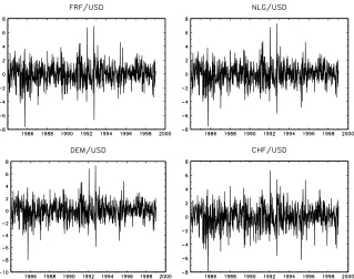
1984 until the end of 1997 (782 observations). As Figure 1 shows, the series exhibit

conditional heteroskedasticity, and against the dollar the rates appear to be relatively

stable. However, the currencies belonging to the European Monetary System (the

French franc, German mark and Dutch guilder) underwent some major realignments

and the foreign exchange markets experienced a number of spells of turmoil during

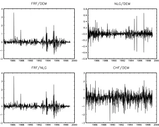
the sample period. These are clearly visible as spikes and excessive volatility in the

implied cross rate returns in Figure 2, whereas the implied cross rates against the

Swiss franc remained quite stable as exemplified by the implied CHF/DEM return series. It is also obvious from Figure 2 that the NLG/DEM ratefluctuates in a much narrower range than the rest.

Let usfirst consider models under normality. We start the analysis by selecting the order of conditional heteroskedasticity,r. A sequential application of test statisticsT1

andT2 as described at the end of the previous section alongside plots of the allegedly

conditionally homoskedastic and heteroskedastic linear combinations of the returns

are employed in the selection process. According to the test results in the upper panel

of Table 1 we cannot reject the null hypothesis of two conditionally heteroskedastic

factors driving the system at the 5% level using either test. In contrast, the hypothesis

of only one factor is easily rejected.

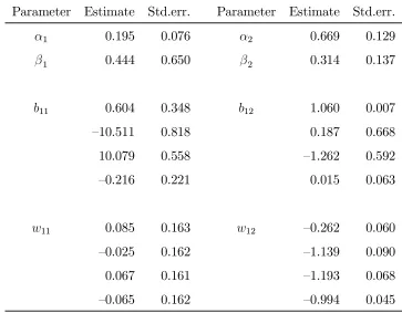
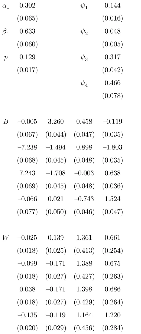
Estimation results for the system with two conditionally heteroskedastic factors

under normality are presented in Table 2. The standard errors and test results to

be reported below are based on the robust covariance matrix estimator, so they are

asymptotically valid even if the assumed normal distribution is not correct.

Interest-ingly, both of the conditionally heteroskedastic factors turn out to be implied exchange

rate returns between European currencies. In the first column of the estimated B1

matrix only the second and third elements are significant at the 5% level. They are approximately equal in absolute value but of opposite sign, suggesting that the first conditionally heteroskedastic linear combination could be the (scaled) difference

be-tween the NLG/USD and DEM/USD returns, i.e., the implied NLG/DEM return.

column of the estimate of B1 only the first and third elements are significant, and

the null hypothesis of the second conditionally heteroskedastic linear combination

being the implied (scaled) FRF/DEM return cannot be rejected by a Wald test

(p-value equals 0.79). However, the coefficients of the first factor in the W matrix are very inaccurately estimated while those of the second factor are clearly significant, suggesting that the one-factor specification might be adequate.

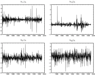
The first conditionally heteroskedastic factor exhibits rather low persistence while the second factor is highly persistent (the estimates of the α and β parameters sum to 0.639 and 0.997, respectively). The heteroskedastic and homoskedastic linear

com-binations of the observed series are depicted in Figure 3. According to these plots

the normality assunption seems to be inadequate for this data set. In particular, the

numerous spikes in these plots indicate excessive kurtosis. This together with the

fact that the coefficients in the estimated W matrix corresponding to thefirst factor have very large standard errors suggests that a model with one factor and nonnormal

error distribution might be a more appropriate specification. It is also noteworthy that the estimatedβ parameter of thefirst factor is insignificant and the estimatedα

parameter of the second factor is clearly greater than the estimate of theβ parameter. Thesefindings suggest that the factors may primarily be driven by ”overreaction” to exceptionally big news and, in turn, lend additional support to the conjecture that

the model may not be appropriate, but a separate regime for these events may be

called for.

Instead of normality a leptokurtic error distribution seems to be needed. One

commonly employed alternative for return series is the t distribution but it turned

out to be inappropriate here. In the model under normality the estimated second

factor primarily seems to capture the rather few outlying observations as attested by

its graph in Figure 3 and the fact that it is dominated by the ARCH term. These

observations lend support to a model in which the errors are generated by two different

distributions of which one generates rather infrequent but large errors. The model

with this idea in mind. Test results for the order of conditional heteroskedasticity

based on this error distribution are presented in the lower panel of Table 1. In this

case the test results are ambiguous at the 5% significance level. Neither test rejects the null hypothesis of two factors (p-values of theT1 andT2 tests equal 0.12 and 0.09,

respectively), while theT1test rejects and theT2 test does not reject the hypothesis of

one factor (p-values equal 0.03 and 0.08, respectively). However, based on the results

of the normal specification above, we are inclined to favor the model with one factor.4 The estimation results of the one-factor model are presented in Table 3, including

the conditionally homoskedastic linear combinations (B2) and corresponding elements

in the W matrix (W2) that are identifiable in this specification. The standard errors

are based on the outer product of the (analytical) score estimator. Because these

standard errors can be badly behaved in finite samples, as recently pointed out by Mencía and Sentana (2004), we use their method of computing the gradient from a

simulated realization of 100,000 observations. The estimates of the elements ofΨare

rather small (in particular less than unity) and the probability or mixing proportion

p is estimated as small as 0.129. This is in accordance with the prior expectation that rather a small error variance prevails most of the time. The conditionally

het-eroskedastic factor exhibits rather moderate persistence (the sum of the estimatedα

andβ parameters equals 0.935) and the GARCH term clearly dominates, suggesting that the introduction of the mixture distribution has successfully captured the

aber-rant observations. The factor in thefirst column of the estimatedB matrix turns out to be the (scaled) difference between the German mark and Dutch guilder returns,

i.e., the implied DEM/NLG return. This hypothesis cannot be rejected by a Wald test

4_TheT

1 andT2tests are essentially tests for conditional homoskedasticity and similar tests have

been shown to overreject in the presence of aberrant observations. As pointed out by Franses et

al. (2004), the problem is especially severe when there are patches of outliers as seems to be the

case here. Moreover, we also attempted to estimate a two-factor model. The estimation algorithm

converged very slowly and, according to Wald tests, only thefirst column of theB1 matrix turned

out to be statistically significant. Thesefindings provide additional support for a model with one

(p-value equals 0.10). In other words, changes in the DEM/NLG rate tend to increase

conditional volatility of the factor. As pointed out above, the range of variation of

the NLG/DEM rate is much narrower than that of the other rates, and it experienced

no realignments during the sample period. Thus, a possible interpretation of the

out-come might be that this particular exchange rate was the most sensitive such that

even its small movements were seen as indicative of changes in market conditions,

giving rise to higher volatility.5 _{According to Wald tests the equation for the French}

franc return is the only one where the conditionally heteroskedastic factor does not

enter (at the 5% significance level). This would imply the rather unexpected finding that there is no dynamics in the conditional variance of the French franc return. As

an additional check for this, we applied a likelihood ratio test. According to this test,

the null hypothesis that the French franc return is not affected by the conditionally

heteroskedastic factor was rejected at any reasonable significance level.

Because all the exchange rates in the system are expressed in terms of the U.S.

dollar, a shock of the same size to all the returns (i.e., to all the elements of εt) can be interpreted as a shocks to the U.S. economy. The coefficients in the first column of W give the effects of the shock on the returns, and as all the estimates except the

one for the DEM/USD return are negative, following a positive shock, the French

franc, Dutch guilder and Swiss franc tend to appreciate vis-à-vis the dollar, while

the German mark tends to depreciate. Also, the coefficients of the NLG/USD and

CHF/USD returns are almost equal while that of the FRF/USD return is clearly

smaller, suggesting substantial appreciation of the Dutch guilder and Swiss franc and

moderate appreciation of the French franc vis-à-vis the German mark. If the shock

is negative the effects are reversed. Moreover, the higher the conditional volatility in

the system, the greater is the impact of such a shock on all the returns.

5_{We also tested for asymmetry by testing whether positive and negative values of the factor have}

equal effect on the conditional variance. A likelihood ratio test cannot reject the null hypothesis of

6 Conclusion

In this paper we extend previous multivariate generalized orthogonal GARCH

mod-els to allow for a reduced number of conditionally heteroskedastic factors. Unlike in

previous similar models we also develop test procedures which can be used to

spec-ify an appropriate number of factors needed to adequately describe the conditional

heteroskedasticity in the data. In addition to Gaussian likelihood, estimation based

on a mixture of normal distributions is also considered. The latter, motivated by

the empirical application of the paper, appears useful when one needs to allow for

aberrant observations, which in our case are due to realignments of the considered

exchange rates.

It is shown that the Gaussian likelihood can be expressed in a convenient form and

its numerical maximization can be facilitated by using simple preliminary estimates.

In large systems such preliminary estimates may also be useful in their own right.

Because in high-dimensional GARCH models full maximum likelihood estimation is,

in general, difficult, our model may thus offer a feasible alternative.

Appendix 1

In this appendix the limiting distributions of test statistics T1(K) and T2(K)

are derived. Unless otherwise stated, all the assumptions stated in the paper will

be assumed, including the correctness of the null hypothesis that the order of

condi-tional heteroskedasticity equalsr. We shall explicitly only consider the case where no column of the parameter matrix B2 is identifiable. The employed arguments can be

straightforwardly modified to other relevant cases.

Derivation of the limiting distribution of T1(K). Let γ∗22(k) be the

coun-terpart of eγ22(k) defined by using y0tB2B20yt = ε20tε2t in place of yt0Be2Be02yt. We start by showing that, for anyfixedk,

e

γ₂₂(k)₋γ∗₂₂(k) =

  

op

¡

T−1/2¢_{, k >0}

op(1), k = 0.

Supposefirst thatk >0and defineξ2t by replacing the estimatorBe2 in the definition

ofeξ_2t byB2. Then we can write

e

γ₂₂(k)₋γ∗₂₂(k) = T−1

T

X

t=k

ξ_2,t−k(eξ_2t−ξ_2t) +T−1

T

X

t=k

ξ_2t(eξ_2,t−k−ξ_2,t−k) (21)

+T−1

T

X

t=k

(eξ2t−ξ2t)(eξ2,t−k−ξ2,t−k).

Using the definitions and assumptions it is straightforward to check that thefirst term on the right hand side can be expressed as

T−1

T

X

t=k

ξ_2,t−k(eξ_2t−ξ_2t) =T−1

T

X

t=k

ξ_2,t−ky0_t(Be2Be20 −B2B20)yt+op

¡

T−1/2¢.

Now define then×nmatricesM =B2R20 andMf=Be2Re02.BecauseMf=Ce−10Re2Re02 =

e

C−10_(I

n−Re1Re01) and because the estimatorsCe andRe1 are assumed to be consistent

of order Op

¡

T−1/2¢_{, we have M}f _{= M +O}

p

¡

T−1/2¢_{. Thus, y}0

t(Be2Be20 −B2B20)yt =

y0

t(MfMf0−M M0)yt= 2yt0M(Mf−M)0yt+yt0(Mf−M)(Mf−M)0yt and

T−1

T

X

t=k

ξ_2,t−k(eξ_2t−ξ_2t) = 2tr(Mf₋M)0T−1

T

X

t=k

ξ_2,t−kytyt0M (22)

+tr(Mf−M)(Mf−M)0T−1

T

X

t=k

ξ2,t−kytyt0 +op

¡

T−1/2¢.

In the second term on the right hand side we can use the definition of ξ_2,t−k to obtain

T−1

T

X

t=k

ξ_2,t−kytyt0 =T−1 T

X

t=k

kε2,t−kk2ytyt0 −T−1 T

X

t=1

kε2tk2T−1 T

X

t=k

ytyt0 =Op(1).

Here the latter equality follows from a law of large numbers because the process

¡

kε2tk2, ytyt0

¢

is stationary and ergodic withfinite second moments. This, in conjunc-tion with the fact Mf₋M = Op

¡

T−1/2¢_{, shows that the second term on the right}

hand side of (22) is of orderop

¡

T−1/2¢_{.To see that the same is true for thefirst term,}

conclude from the definitions that y0

tM = ε0tH

1/2

definition of ξ2,t−k and equation (9) it follows that

T−1

T

X

t=k

ξ_2,t−kytyt0M = T−1 T

X

t=k

Ã

kε2,t−kk2−T−1 T

X

t=1

kε2tk2

!

W1Vt1/2ε1tε02tR20(23)

+T−1

T

X

t=k

Ã

kε2,t−kk2−T−1 T

X

t=1

kε2tk2

!

W2ε2tε02tR02.

It is easy to check that on the right hand side the replacement of the sample mean

T−1PT

t=1kε2tk2 by its expected valuen−r causes an error of order op(1)and, after this replacement, the resulting summands are in both cases realizations from zero

mean stationary and ergodic processes. Thus, both terms on the right hand side of

(23) are of order op(1)and, since Mf−M =Op

¡

T−1/2¢_{, the first term on the right}

hand side of (22) is of orderop

¡

T−1/2¢_.

Altogether we have shown that the first term on the right hand side of (21) is of order op

¡

T−1/2¢_{. By similar arguments it can be seen that the same is true for the}

second and third terms. For the second term this essentially amounts to considering

(22) withk <0whereas the third term is clearly of a lower order of magnitude. Hence, we have established (20) whenk >0. The casek = 0 can be handled similarly.

Now recall that γ∗₂₂(k) is the kth sample serial covariance obtained from kε2tk2,

(t= 1, ..., T). Thus, well-known results about stationary time series show that the corresponding sample serial correlations γ∗₂₂(k)/γ∗₂₂(0) are asymptotically indepen-dent and normally distributed with mean zero and variance1/T. From (20) it readily follows that the same is true for the corresponding observed quantitieseγ22(k)/eγ22(0).

The limiting distribution of test statistic T1(K)follows from this.

Derivation of the limiting distribution of T2(K). We consider analogues

of the sample serial covariance matrices eΓ(k) defined by replacing the half vector-ization operator vech by the ordinary vectorvector-ization operator vec. Thus, set eζ_2t =

vec(Be0

2ytyt0Be2)−T−1

PT

t=1vec(Be20yty0tBe2), and define

e

Γ(k) =T−1

T

X

t=k

eζ

2teζ 0

and Γe(k) = eΓ(−k)0 for T < k < 0. The unobserved counterparts of eζ_2t and Γe(k)

obtained by replacing the estimator Be2 byB2 are denoted by ζ₂∗_t andΓ∗(k),

respec-tively. In order to simplify notation we denote wt = wt−T−1PTt=1wt for any time series vector wt (t = 1, ..., T) andA(2) =A⊗A for any matrix A. Various results of the Kronecker product and the vectorization operator to be used below can be found

in Sections 2.4 and 7.2 of Lütkepohl (1996).

Analogously to (20) we first show that, for any fixedk,

e

R(2)₂ Γe(k)Re(2)₂ 0 −R(2)₂ Γ∗(k)R(2)₂ 0 =

  

op

¡

T−1/2¢, k >0

op(1), k = 0.

(24)

By properties of the vec operator, vec(Be0

2yty0tBe2) = Be

(2)0

2 y (2)

t . Hence, eζ_2t = Be

(2)0

2 y (2)

t

andΓe(k) =Be₂(2)0Γe(2)_y (k)Be₂(2) where eΓ_y(2)(k) =T−1PT t=ky

(2)

t y

(2)0

t−k.In the same way it can be seen that Γ∗(k) =B(2)₂ 0eΓ(2)_y (k)B(2)₂ .

Considerfirst the casek > 0.Using the matricesM andMfdefined in the previous proof we can write

e

R(2)₂ Γe(k)Re(2)₂ 0₋R(2)₂ Γ∗(k)R(2)₂ 0 = Mf(2)0Γe(2)_y (k)Mf(2)₋M(2)0eΓ(2)_y (k)M(2) (25)

= (Mf(2)₋M(2))0Γe(2)_y (k)M(2)

+M(2)0eΓ(2)_y (k) (Mf(2)₋M(2))

+(Mf(2)₋M(2))0Γe_y(2)(k) (Mf(2)₋M(2)).

Because the process yt is stationary and ergodic with finite fourth moments, a law of large numbers implies that Γe(2)_y (k) =Op(1). This, in conjunction with the result

f

M −M = Op

¡

T−1/2¢_{, shows that the last term in the last expression of (25) is of}

order op

¡

T−1/2¢_{. We show that the this is also the case for thefirst term.}

From the identity

f

it follows that

(Mf(2)₋M(2))0Γe(2)_y (k)M(2) = (M0 _⊗(Mf₋M)0)eΓ(2)_y (k)M(2)

+((Mf₋M)0_⊗M0)eΓ(2)_y (k)M(2)

+(Mf₋M)(2)0Γe(2)_y (k)M(2).

As noticed above, eΓ(2)_y (k) = Op(1) which in conjunction with the result Mf−M =

Op

¡

T−1/2¢_{implies that the last term on the right hand side of the preceding equation}

is of order op

¡

T−1/2¢_{. Thus, we need to show that the same is true for the first and}

second terms. It suffices to consider the former which can be expressed as

(M0⊗(Mf−M)0)eΓ(2)_y M(2) = (M0⊗(Mf−M)0)T−1

T

X

t=k

y(2)t y

(2)0 t−kM(2)

= (In⊗(Mf−M)0)T−1 T

X

t=k

¡

M0_y t⊗yt

¢ ¡

M0_y

t−k⊗M0yt−k

¢0

= (In⊗(Mf−M)0)T−1 T

X

t=k

¡

R2ε2t⊗yt

¢ ¡

R2ε2,t−k⊗R2ε2,t−k

¢0

.

Here the last equality is based on the fact M0_y

t =R2ε2t already used in the previous proof. Because the processR2ε2t⊗ytis stationary and ergodic withfinite expectation it obeys a law of large numbers. Using this fact in conjunction with Mf− M =

Op¡T−1/2¢ it is not difficult to check that the replacement of the sample mean in the last expression above by the corresponding expectation causes an error of order

op

¡

T−1/2¢_{. Thus,}

(M0⊗(Mf−M)0)eΓ(2)y (k)M(2)

= (In⊗(Mf−M)0)T−1 T

X

t=k

(R2ε2t⊗yt−E(R2ε2t⊗yt))

×(R2ε2,t−k⊗R2ε2,t−k−E(R2ε2,t−k⊗R2ε2,t−k))0 +op

¡

T−1/2¢.

are stationary and ergodic martingale differences and, hence, of order op(1). Thus, becauseMf₋M =Op

¡

T−1/2¢_{it follows thatM}0_⊗(Mf_−M)0_Γe(2)

y (k)M(2) =op

¡

T−1/2¢_.

We have thus shown that the first term in the last expression of (25) is of order

op

¡

T−1/2¢_{. A similar proof shows that this is also the case for the second term. The}

proof is essentially based on arguments used above with k < 0. Altogether we have shown that, for k > 0, all the three terms in the last expression of (25) are of order

op

¡

T−1/2¢_{. This proves (24) in the casek > 0. The case k = 0 can be obtained from}

(25) by using the facts Γe(2)_y (k) =Op(1)andMf−M =Op

¡

T−1/2¢_.

We shall next obtain an alternative expression for test statistic T2(K). To this

end, letA+ _{signify the Moore-Penrose inverse of the matrixA. Then, we can write}

T2(K) = T

K

X

k=1

tr³Re(2)2 Γe(k)Re (2)0

2

´0³

e

R(2)2 eΓ(0)Re (2)0

2

´+

(26)

׳Re(2)₂ Γe(k)Re(2)₂ 0´ ³Re(2)₂ Γe(0)Re(2)₂ 0´+.

In order to justify this, conclude from the definitions of the vectors eζ_2t and eζ_2t that

e_ζ

2t = Dn−reζ2t and eζ2t =D

+

n−reζ_2t where Dn+−r =

¡

D0

n−rDn−r

¢−1

D0

n−r. Thus, eΓ(k) =

Dn−reΓ(k)D0n−r and eΓ(k) = D+n−rΓe(k)D+n−0r. From these facts and the definition of the Moore-Penrose inverse it can be straightforwardly shown that³Re(2)2 Γe(0)Re

(2)0

2

´+ =

e

R(2)₂ D+n−0rΓe(0)−1Dn+−rRe

(2)0

2 . Using this identity and the fact Re (2)0

2 Re (2)

2 = In−r on the right hand side of (26) it can then be seen that the stated equation holds.

Next note that from the definitions it follows that Γ∗(k) is the sample serial co-variance matrix of the random vector ε2t⊗ε2t at lag k. Thus, by standard results,

R(2)₂ Γ∗(0)R(2)₂ 0 converges in probability to R(2)₂ Cov(ε2t⊗ε2t)R(2)2 0 and, by (24), the

same is true forRe(2)2 Γe(0)Re (2)0

2 .The rank of the covariance matrix Cov(ε2t⊗ε2t)is not full but(n₋r) (n₋r+ 1)/2or the rank of the covariance matrix Cov¡Dn+−r(ε2t⊗ε2t)

¢

(cf. the relations eζ2t = D+n−reζ_2t and eΓ(k) = D+n−rΓe(k)Dn+−0r discussed above). Be-cause the matrix R(2)₂ satisfies R₂(2)0R(2)₂ = In−r the rank of R(2)2 Cov(ε2t⊗ε2t)R(2)2 0

is also (n−r) (n−r+ 1)/2 and because Re(2)2 Γe(0)Re (2)0

2 = R (2)

2 Cov(ε2t⊗ε2t)R(2)2 0 +

op(1) we must have rk

³ e

approaching one (cf. the proof of Lemma 1 in Andrews (1987)). On the other

hand, because the structure of the matrix Re(2)₂ Γe(0)Re(2)₂ 0 is similar to that of the matrix R(2)₂ Cov(ε2t⊗ε2t)R(2)2 0 it follows that the inequality rk

³ e

R(2)₂ Γe(0)Re(2)₂ 0´ ≤

(n₋r) (n₋r+ 1)/2 must hold. Thus, with probability approaching one the rank of the matrix Re(2)₂ Γe(0)Re(2)₂ 0 equals (n−r) (n−r+ 1)/2, the rank of its probability limit R₂(2)Cov(ε2t⊗ε2t)R(2)2 0. From Theorem 2 of Andrews (1987) we therefore find

that

³ e

R(2)₂ eΓ(0)Re(2)₂ 0´+ = ³R(2)₂ Cov(ε2t⊗ε2t)R(2)2 0

´+

+op(1) (27)

= R₂(2)D_n+₋0_r¡Cov(D_n+_−r(ε2t⊗ε2t))

¢−1

D+_n−rR(2)₂ 0+op(1).

Here the latter equality can be justified by using the definition of the Moore-Penrose inverse (cf. the expression obtained for³Re(2)₂ Γe(0)Re(2)₂ 0´+ after (26)). Thefirst equal-ity also holds with the left hand side replaced by ³R(2)₂ Γ∗(0)R(2)₂ 0´+.

As will become clear below, T1/2_R(2)

2 Γ∗(k)R (2)0

2 = Op(1) for k > 0. This in con-junction with equations (24), (26) and (27) yields

T2(K) = T

K

X

k=1

tr³R(2)₂ Γ∗(k)R(2)₂ 0´0³R(2)₂ Γ∗(0)R(2)₂ 0´+

׳R(2)₂ Γ∗(k)R(2)₂ 0´ ³R(2)₂ Γ∗(0)R(2)₂ 0´++op(1)

= T

K

X

k=1

trΓ∗(k)0Γ∗(0)−1Γ∗(k)Γ∗(0)−1+op(1),

whereΓ∗_{(k)is the sample serial covariance matrix ofD}+

n−r(ε2t⊗ε2t)at lag kand the latter equality follows from (27) with arguments similar to those used for (26). The

limiting distribution of test statistic T2(K)can be derived from this.

To complete the proof, denoteet =D+n−r(ε2t⊗ε2t)andF∗(k) =Γ∗(0)−1/2Γ∗(k)Γ∗(0)−1/2. By standard arguments it can first be seen that

Γ∗(k) =T−1

T

X

t=k

(et−Eet) (et−k−Eet−k)0+op

¡

T−1/2¢ (k > 0).

This and a standard application of a martingale central limit theorem show that the

variates and, moreover, these limits are independent fork = 1, ..., K.Thus, it follows that T2(K) = T PK_k=1trF∗(k)F∗(k)0+op(1)→d χ2

¡

K(n₋r)2(n₋r+ 1)2/4¢.

Appendix 2

Derivatives of the Gaussian log-likelihood function. For numerical

op-timization and estimation of the matrices Q0 and Q1 in the limiting distributions

(16), (17) and (18) it is useful to have analytical expressions of the first and second derivatives of the Gaussian log-likelihood function. It will be convenient to consider

the log-likelihood of a single observation which, by the expression of the conditional

density function (12) and the subsequent discussion, can be written as

¯

lt(Φ, R1, δ) = log det (Φ)− 1 2y

0 tΦ0Φyt − r X i=1 µ 1

2logvit− 1 2(v

−1

it −1)(ρ 0

1iΦyt)2

¶

def

= ¯l0t(Φ) + r

X

i=1 ¯

lit(Φ, ρ1i, δi).

With this parameterization, equation (6) can be written as

vit = (1−αi −βi) +βivi,t−1+αi(ρ01iΦyt−1)2 i= 1, ..., r.

Note also that the formulation of some of the subsequent results assume that the

parameter matrix Φ is symmetric although the transpose sign is not suppressed

from the notation. The parameters of the model are collected in the vector θ = [φ0 ρ0

11 · · · ρ01r δ 0

1 · · · δ

0 r]

0

where φ =vech(Φ).

By straightforward differentiation,

∂¯l0t(θ)/∂φ=D0nvec(Φ−1)−

1 2D

0

nvec(ytyt0Φ0)−

1 2D

0

nvec(Φyty0t) (28) and, for 1_≤i_≤r,

∂¯lit(θ)/∂φ = −

1 2v

−1

it (∂vit/∂φ) +

1 2v

−2