Evaluation on GA based Model for solving JSSP

Evaluation on GA based Model for solving JSSP

A. Tamilarasi

Professor and Head, Dept. of MCA

Kongu engineering college, Erode, TN, India

S. Jayasankari

Assistant Professor Dept. of MCA

VIIMS, Tiruchengode, TN, India

ABSTRACT

The optimization techniques such as Genetic algorithm (GA), Particle Swarm Optimization (PSO), Ant Colony Optimization (ACO), Simulated Annealing (SA), etc., were commonly used in solving job shop scheduling problem (JSSP). There are different variants of these algorithms that were addressed in several previous works. In previous literatures, it was commonly mentioned that the initial solution were generally guessed in a very random manner (such as random initialization of population in GA). In this work, we will address the impact of such random initialization on solving the JSSP while using an optimization technique - GA. The performance of this algorithm will be evaluated with different set of initial conditions. In one experiment, during initialization stage, the initial population will be initialized with random schedules. In another experiment, the initial population will be initialized with a known, worst case schedule. The impact of this initial condition on the performance of algorithm has been studied and achieved makespan. The arrived results proved that the conventional way of randomly selecting initial conditions of the evolutionary process has a worst effect on performance in JSSP of higher dimensions. While initializing with known, worst case solution, the evolutionary process was capable of converging into meaningful and more optimum solutions.

Keywords

Scheduling, Job Shop Scheduling, Genetic Algorithm, Gant-Chart.

1.

INTRODUCTION

In the modern competitive environment in manufacturing and service industries, the effective sequencing and scheduling has become an essential for survival in the marketplace [6]. Companies have to produce their product untimely as opposed to due date. Otherwise, it will impinge upon reputation of a business. At the same time, the activities and operations need to be scheduled with the intention that the available resources will be used in an efficient manner. As a result, there is a great good scheduling algorithm and heuristics are invented. Most of the prevailing practical scheduling problems exist in stochastic and dynamic environment.

Stochastic is a problem where some of the variables are uncertain while dynamic problem is when jobs arrive randomly. On the other hand, the problems with ready time is known and fixed are called problems static and for problem where all the parameter such as processing times are known and fixed is called deterministic problems (French, 1982). In spite of this, it is quite impossible to predict exactly when jobs will become available for processing. Additionally, the understanding of scheduling problems where there is no

uncertainty involved will help us towards the solution of stochastic and dynamic problems.

The main objective in solving the job shop scheduling problem is to find the sequence for each operation on each machine that optimizes the objective function. The most common objective function that has been used in scheduling the job shop problem is minimization of makespan value or the time to complete all jobs. It has been the principal criterion for academic research and is able to capture the fundamental computational difficulty which exists unconditionally in determining an optimal schedule (Jain and Meeran, 1999).

1.1

The Types of Related Scheduling

Problems

We can group the main classical scheduling problems in five distinct classes:

 Workshops with only one machine: There is only one machine which must be used for scheduling the given jobs, under the specified constraints.

 Flow shop: There is more than one machine and each job must be processed on each of the machines - the number of operations for each job is equal with the number of machines, the jth operation of each job being processed on machine j.

 Job shop: The problem is formulated under the same terms as for the flow shop problem, having as specific difference the fact that each job has associated a processing order assigned for its operations.

 Open shop: The same similarity with the flow shop problem, the processing order for the operations being completely arbitrary the order for processing a job's operations is not relevant; any ordering will do.

 Mixed Workshop: There is a subset of jobs for which a fixed processing path is specified, the other jobs being scheduled in order to minimize the objective function.

1.2 Problem Definition

In the following way, the job shop scheduling problem (JSSP) will be described: For „n‟ jobs, each one is composed of several operations that must be executed on „m‟ machines. For each operation uses only one „m‟ machines for a fixed duration. Each machine can process at most one operation at a time and once an operation starts processing on a given machine, it must complete processing on that same machine without any interruption. The operations of a given job have to be processed in a given set of order. The problem is to find out a schedule of the operations on the machines, taking into an account the precedence constraints, that minimizes the makespan (Cmax), ie, the

finishing time of the all the operations completed within the scheduled time.

We focus on job-shop scheduling problems composed of the following elements [4]:

 Jobs: J = {J1, • • •, Jn } is a set of n jobs to be

scheduled. Each job Ji consists of a predetermined

sequence of operations. Oi,j is the operation j of Ji.

All jobs are released at time 0.

 Machines: M = {M1 , • • •, Mm } is a set of m

machines. Each machine can process only one operation at a time. And each operation can be processed without interruption during its performance on one of the set of machines. All machines are available at time 0.

 Constraints: The constraints are rules that limit the possible assignments of the operations. They can be divided mainly into following situations:

- Each operation can be processed by only one machine at a time (disjunctive constraint). - Each operation, which has started, runs to completion (non-preemption condition). - Each machine performs operations one after another (capacity constraint).

- Although there are no precedence constraints among operations of different jobs, the

predetermined sequence of operation for each job forces each operation to be scheduled after all predecessor operations (precedence/conjunctive constraint).

- The machine constraints emphasize the operations can be processed only by the machine from the given set (resource constraint).

 Objective(s): Most of the research reported in the literature is focused on the single objective case of the problem, in which the objective is to find a schedule that has minimum time required to complete all operations (minimum makespan). Some other objectives, such as flow time or tardiness are also important like the makespan.

1.3

Different Approaches for Solving

Scheduling Problems

Job-shop scheduling problem is one of the well-known and hardest combinatorial optimization problems. During the last three decades, this problem has captured the interest of a significant number of researchers.

The JSSPs are well-known combinatorial optimization problems, which consist of a finite number of jobs and machines. Each job consists of a set of operations that has to be processed, on a set of known machines, and where each operation has a known processing time.

A schedule is to be complete a set of operations, required by a job, to be performed on different machines, in a given order. In addition, the process may need to satisfy other constraints such as (i) no more than one operation of any job can be

executed simultaneously and (ii) no machine can process more than one operation at the same time. The objectives usually considered in JSSPs are the minimization of makespan, the minimization of tardiness, and the maximization of throughput. The total time elapsed between the starting of the first job‟s first operation and the ending of the last operation, is termed as the makespan.

In JSSPs, the size of the solution space is an exponent of the number of machines, which makes it quite expensive to find the best makespan for larger problems. By larger problem, we mean a higher number of jobs and (or) a higher number of machines. Most JSSPs that have appeared in the literature are for ideal conditions.

However, in practice, process interruptions like machine breakdown and machine unavailability are very common, which makes JSSPs more complex to solve. There exist a variety of conventional optimization methods for solving JSSPs, such as the integer programming method. However, the conventional methods are unable to solve larger problems due to the limitation of current computational power. Considering the complexity of solving JSSPs, with or without interruptions, and the limitations of existing methodologies, it seems that an evolutionary computation based approaches would do better, as they have proven to be successful for solving many other combinatorial optimization problems. Job shop scheduling is naturally a NP-hard problem with no easy solution. Branch-and-bound, Tabu search, and biologically stimulated approaches such as GA, Swarm Intelligence and other stochastic model such as Simulated Annealing algorithm were proposed for achieving possible solutions to complex problems such as job shop scheduling. During the last few decades, Evolutionary Computing (EC) has emerged as an authoritative methodology for managing the often highly complex problems of modern society, such as optimizing engineering design, job shop scheduling, and transport systems. Such real-world optimization problems typically are characterized by huge, ill-behaved solution spaces which are not feasible to exhaustively search and defy traditional optimization algorithms because they are for instance non-linear, non-differentiable, non-continuous, or non-convex [3]. EC encompasses a class of stochastic, population-based, optimization algorithms inspired by biological evolution and genetics which have been shown to perform well on problems with huge, ill-behaved solution spaces.

Job Shop Problem has been basically considered using the following approaches [5]:

 Exact methods: Giffler and Thompson (1960), Brucker et al. (1994) and Williamson et al. (1997)  Branch and bound: Lageweg et al. (1977), Carlier

and Pinson (1989, 1990), Applegate and Cook (1991) and Sabuncuoglu and Bayiz (1999). Carlier and Pinson (1989) have been successful in solving the notorious 10´10 instance of Fisher and Thompson proposed in 1963 and only solved twenty years later; Heuristic procedures based on priority rules: French (1982), Gray and Hoesada (1991) and Gonçalves and Mendes (1994)

 Shifting bottleneck: Adams et al. (1988). Problems of dimension 15´15 are still considered to be beyond the reach of today's exact methods. Over the last decade, a growing number of metaheuristic procedures have been presented to solve hard optimization problems[5]:

 Tabu Search: Taillard (1994), Lourenço and Zwijnenburg (1996) and Nowicki and Smutnicki (1996)

 Genetic Algorithms: Davis (1985), Storer et al. (1992), Aarts et al. (1994), Croce et al. (1995), Dorndorf et al. (1995), Gonçalves and Beirão (1999) and Oliveira (2000).

Additionally, some researchers have developed local search procedures: Lourenço(1995), Vaessens et al. (1996), Lourenço and Zwijnenburg (1996) and Nowicki and Smutnicki (1996). Surveys of heuristic methods for the JSP are given in Pinson (1995), Vaessens et al. (1996) and Cheng et al. (1999).

A survey of Job Shop Scheduling techniques can be found in Jain and Meeran (1999). Recently Wang and Zheng (2001) developed a Hybrid Optimization strategy for JSP, Binato et al. (2002) present a greedy randomized adaptive search procedure (GRASP) for JSP and Aiex et al. (2003) introduced a parallel GRASP with path-relinking for JSP.

2.

THE JSSP AND MODELS

CONSIDERED FOR SOLVING JSSP

2.1 Mathematical Representation of the

JSSP

Let J = {0, 1, …, n, n+1} denote the set of operations to be scheduled and M = {1,..., m} the set of machines. The operations 0 and n+1 are not original, and they have no duration and represent the initial and final operations. The operations are interrelated by two types of constraints. First, the precedence constraints, which force each operation j to be scheduled after all predecessor operations, Pj, are

completed. Second, operation j can only be scheduled if the machine it requires is idle. Further, let dj denote the

(fixed) duration (processing time) of operation j.

Let Fj represent the finish time of operation j. A schedule can

be represented by a vector of finish times (F1, , Fm, ... , Fn+1).

Let A(t) be the set of operations being processed at time t, and let rj,m = 1 if operation j requires machine m to be processed

otherwise rj,m = 0.

The model of the JSP can be described the following way[5]:

Minimize Fn+1 (Cmax) ……….(1)

Subject to:

Fk ≤ Fj – dj j-1,…,n+2 ; k ϵ Pj ……….(2)



r



Fj ≥ 0 j=1,….,n+1 ……….(4)

The objective of function is to (1) minimize the finishing time of operation n+1 (the last operation), and minimizes the makespan. Constraints (2) impress the precedence relations between operations and constraints (3) state that one machine can only process one operation at a time. Finally (4) forces the finishing time to be non- negative.

2.2 Genetic Algorithm (GA)

Genetic Algorithms (GAs) are known as Evolutionary Algorithms used in regular practice. GAs and other EAs are

population based search techniques that explore the solution space in a discrete manner. In this algorithm, the solutions evolve by applying reproduction operators. When GAs/EAs are hybridized with local search, they are known Memetic Algorithms (MAs).

The priority rules are widely used in the scheduling area for either problem solving or refinement of solutions with another technique. In solving JSSPs, the priority rules can be used as local search in conjunction with genetic algorithms, which is basically a memetic algorithm. These approaches have been proved to be efficient for solving job-shop scheduling problems.

Genetic algorithms are adaptive methods, which may be used to solve search and optimization problems (Beasley et al. (1993)). They are based on the genetic process of biological organisms. Over many generations, natural populations evolve according to the principles of natural selection, i.e. survival of the fittest, first clearly stated by Charles Darwin in The Origin of Species. By mimicking this process, genetic algorithms are able to evolve solutions to real world problems, if they have been suitably encoded.

Before a genetic algorithm can be run, a suitable encoding (or representation) for the problem must be devised. A fitness function is also required, which assigns a figure of merit to each encoded solution. During the run, parents must be selected for reproduction, and recombined to generate offspring.

It is assumed that a potential solution to a problem may be represented as a set of parameters. These parameters (known as genes) are joined together to form a string of values (chromosome). In genetic terminology, the set of parameters represented by a particular chromosome is referred to as an individual. The fitness of an individual depends on its chromosome and is evaluated by the fitness function.

The individuals, in the reproductive phase, are selected from the population and recombined, producing offspring, which comprise the next generation. Parents are randomly selected from the population using a scheme, which favors fitter individuals. Having selected two parents, their chromosomes are recombined, typically using mechanisms of crossover and mutation. Mutation is usually applied to some individuals, to guarantee population diversity. The general form of genetic algorithm is as follows:

Genetic Algorithm {

Generate initial population Pt

Evaluate population Pt

While stopping criteria not satisfied Repeat {

Select elements from Pt to copy into Pt+l Crossover

elements of Pt and put into Pt+l Mutation elements

of Pt and put into Pt+l Evaluate new population Pt+l

Pt = Pt+l

} }

3.

THE REPRESENTATION OF JSSP

SOLUTIONS

Definition 1. String Representation.

Consider three finite sets, a set J of jobs, a set M of machines and a set O of operations. For each operation a there is a job j(a) in J to which it belongs, a machine m(a) in M on which it should be executed and a processing time d(a). For each operation a its successor in the job is given by sj(a), except for the last operation in a job. The representation of a solution is a string consisting of a permutation of all operations in O, that is an element of the set:

StrRep = { s belongs to On | n = |O| and for all i, j with 1 ≤ i

< j ≤ n: s(i) ≠ s(j) } ……..(7) Now we can define legal strings. Formal for s in StrRep: Legal(s) = For all a, sj(a) belongs to O: a ~< sj(a) ……..(8) where a ~< b means: a occurs before b in the string s.

Theorem 1. (Feasible Solution → Legal String)

Each and every feasible solution can be represented by a legal string. And one legal string corresponding to the same feasible solution may exist.

Theorem 2. (Legal String → Feasible Solution)

Every legal string corresponds exactly to one feasible solution.

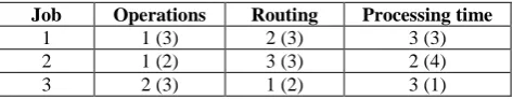
To explain the JSSP and a valid/legal and invalid/illegal solutions, we have chosen the simplest 3x3 JSSP presented in [10]. This example of a 3x3 JSSP is given in Table1. The data includes the routing of each job through each machine and the processing time for each operation in parentheses. For example, “2(3)” in the third row represents the operation one of the Job 3 and the 2 in “2(3)” represents that that operation should be scheduled to machine 2 and the operation will consume 3 units of time.

Table 1 : A 3x3 JSSP

Job Operations Routing Processing time

1 1 (3) 2 (3) 3 (3)

2 1 (2) 3 (3) 2 (4)

3 2 (3) 1 (2) 3 (1)

The one of the known optimum schedule of the above problem is [ J1,1, J3,1, J2,1, J1,2, J3,2, J2,2, J2,3, J1,3, J3,3 ].Here, for

example, J1,2 represents the operation 2 of the Job 1.

Figure1shows one of such a optimum solution for the problem represented by “Gantt-Chart".

Figure 1 : The Gantt-Chart Representation of the Solution of the above 3x3 Problem

If we denotes the operations of the job as follows,

Job1: Op1, Op2, Op3 Job2: Op4, Op5, Op6 Job3: Op7, Op8, Op9

Or simply 1 2 3 4 5 6

7 8 9

then, the schedule [ J1,1, J1,2, J1,3, J2,1, J2,2, J2,3, J3,1, J3,2, J3,3] or

simply [1, 2, 3, 4, 5, 6, 7, 8, 9] will be the one of the known worst case schedule which will satisfy all the conditions of the JSSP. But in this case, the makespan will not be optimum. The schedule [ J1,1, J3,1, J2,1, J1,2, J3,2, J2,2, J2,3, J1,3, J3,3 ] or

simply [1, 7, 4, 2, 8, 5, 6, 3, 9] will be the one of the best know optimum solution. Here the strings “1, 2, 3, 4, 5, 6, 7, 8, 9” and “1, 7, 4, 2, 8, 5, 6, 3, 9” represents solutions and known as valid strings.

In GA, a legal string or a illegal string (of numbers) which represent the order of the schedule can be represented by a chromosome. For example, the known worst case solution can be represented as a chromosome of GA by a string “1, 2, 3, 4, 5, 6, 7, 8, 9” . Similarly, the chromosome of GA “1, 7, 4, 2, 8, 5, 6, 3, 9” will represent a legal string which is an optimal solution of JSSP.

And for example, the chromosome “3, 9, 4, 2, 1, 5, 6, 7, 8” will be an invalid string which correspond to an illegal operation or schedule since this schedule will not satisfy the conditions of JSSP.

So, if we select the initial chromosomes of GA or initial points of SOP with random values, then there will be lot of invalid strings in the initial guessing values. The scope of the evolutionary algorithm is to permute the most optimal string to better most optimal string which will hopefully make that string as a legal string in proceeding generations/steps and finally we will end up with a string belongs to a better solution or optimal schedule with minimum makespan. This assumption will be good and can produce meaningful solutions for lower order scheduling problems such as 3x3 JSSP or 4x4 JSSP. But, it may produce illegal solutions even after very long runs in the case of higher order scheduling problems like 15x15 JSSP. Because, if we randomly chose initial population then there will be much chance for getting all illegal strings in the initial set which belongs to no nearby solution. So the fitness calculation methods will lead to meaningless fitness values and the selection method will also be incapable of selecting a better solution in each generation or step. So in each step of the evolutionary process there will not be any guaranty of getting progressive solution.

So we believe that the random selection of initial solution/seed in an evolutionary algorithm will not lead to a better result in higher order scheduling problems such as 15x15 JSSP. So in this work, we have evaluated the performance of evolutionary optimization technique GA with different initial conditions.

4.

RESULTS AND ANALYSIS

In the experiment, we have randomly chosen the initial conditions as in the traditional evolutionary method. We expect that, it will be capable of producing at latest one meaningful legal string in every generation/step and hence there will be a much good probability of achieving a better solution in the succeeding generations or steps.

4.1 Analysis of Performance with Different

Problem Size

The Analysis with 3x3 JSSP

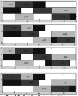
In fact, in small JSSP problems, we did not expect any difference in behavior. But, while running the GA based algorithm, the algorithm found different optimum solutions with same best makespan.

In the following figures we are presenting the Gantt-Chart found by the GA based method for the 3x3 problem[10] presented in table 1. In the following schedules, the forth one is solution already discussed in figure 1. The code developed for drawing Gantt-Chart will display the chart in color. But here we displayed the output of 3x3 as a gray image for better visibility.

Figure 2: The Gantt-Chart Representation of the

Solutions found by GA based algorithm for the previously mentioned 3x3 Problem

4.2 The Analysis with Higher Dimensional

JSSP

With the problems of lower dimensions, there was not much noticeable difference in convergence process, in this type of initialization if initial condition of the evolutionary process. But, while solving higher dimensional problems, the impact was more obvious. To minimize the time, we have chosen very low number of generations/steps. So the final fitness will not be the ideal and more optimum result. Even though the Gantt-Charts attained were not optimal, but they were not illegal solutions. But in the case of random initialization, the algorithm only produced illegal solutions up to that 100 generations/steps.

The Analysis with 6x6 JSSP Result with Random Initialization

Due to random initialization, the fitness stares from a worst value 3.5x106(avg.) and 10x105 (min).

Figure 3 : Gantt-Chart

Results of Initialization with Worst Case Solution

As shown in the following Gantt-Chart, the initialization with worst case solution produced better results. Due to the meaningful worst case initialization, the fitness stares from a meaningful value 160 (min) and the mean value also fall between zero and 3x105 (avg).

Figure 4 : Gantt-Chart

Performance in terms of speed

To measure the performance in terms of speed, with problems of different sizes, the model was run with problems of different sizes.

Table 2 : The time taken for different JSSP size

Sl.No JSSP Size Time Taken(sec) GA

1 3x3 4.14

2 4x4 5.06

3 6x6 8.39

4 10x10 25.02

5 15x15 89.45

Convergence Capability of the Algorithms

The convergence property was also measured with problems of different sizes and tabulated below.

Table 3: Startup with known worst case solution

Sl.No

JSSP Achieved Optimal

Solution (Makespan)

Size Known best

optimum value GA

2 4x4 272 272

3 6x6 55 68

4 10x10 902 2214

5 15x15 1268 6771

Even though the arrived solution is far from the optimal solution (since we run this for low generations), the better performance in the case of GA is very obvious.

5.

CONCLUSION

We have successfully implemented the basic evolutionary model for solving JSSP using GA. The arrived results show that the models produced optimal or near-optimal solutions medium level job shop scheduling problems. Even the system was capable of finding more than one solution with same makespan value.

The arrived result proves that the conventional way of randomly selecting initial conditions of the evolutionary process has a worst effect on performance in JSSPs of higher dimensions. While initializing with known, worst case solution, the evolutionary process was capable of converging into meaningful and more optimum solutions. GA was capable of finding more than one better solution from the problem space.

6. FUTURE WORK

In this work, we have just selected the evolutionary algorithms based on their popularity. There are few more algorithms of the same kind exists. Future works may address the impact of the selection of initial condition in those algorithms also. We observed that the overall performance lack of this kind of evolutionary algorithm is due to the illegal strings appeared again and again during the evolutionary process. Lot of time is unnecessarily wasted to identify a string as illegal and eliminating it from further processing. Future works may address evolutionary techniques which will avoid even the generation of illegal strings during the evolutionary process. A new kind of mutation and crossover operation may be developed to avoid the production of illegal strings or solutions to make GA exclusively suitable for JSSP.

7.

ACKNOWLEDGEMENTS

Our sincere thanks to our management Kongu Engineering College, Vivekanadha Institutions for Women, and the innovative members who helped us towards the development of this research paper come in a successful way.

8.

REFERENCES

[1] Moraglio , H.M.M. Ten Eikelder, R. Tadei, “Genetic Local Search for Job Shop Scheduling Problem”, Technical Report, CSM-435 ISSN 1744-8050.

[2] E.L. Lawler, J.K. Lenstra, A.H.G. Rinnooy Kan, D.B. Shmoys. - Sequencing and scheduling:

Algorithms and complexity. - In: S.C. Graves, A.H.G. Rinnoy Kan and P. Zipkin, editors, Handbooks in Operations Research and Management Science 4, North- Holland, 1993.

[3] Dr. Daniel Tauritz, The abstract of the talk "Grand Challenges in Evolutionary Computing - Part II", Missouri S&T .

[4] Hongbo Liu, Ajith Abraham,Zuwen Wang, "A Multi-swarm Approach to Multi-objective Flexible Job-shop Scheduling Problems", School of Information Science and Technology, Dalian Maritime University, Dalian 116026, China, Fundamenta Informaticae,IOS Press, 2009.

[5] José Fernando Gonçalves, Jorge José de Magalhães Mendes,Maurício G. C. Resende, “A Hybrid Genetic Algorithm for the Job Shop Scheduling Problem”, AT&T Labs Research Technical Report TD-5EAL6J, September 2002.

[6] Mahanim Binti Omar, “A Modified Multi-Step Crossover Fusion (Msxf) In Solving Some Deterministic Job Shop Scheduling Problem (Jssp), A thesis work submitted to Universiti Sains Malaysia, 2008.

[7] Puspa MahatPuspa Mahat, "Swarm Intelligence and Machine Learning", Xiangyang Wang, Jie Yang, Richard Jensenb Xiaojun Liu, , "Rough Set Feature Selection and Rule Induction for Prediction of Malignancy Degree in Brain Glioma ", Institute of Image Processing and Pattern Recognition, Shanghai Jiao Tong University, Shanghai, China and Department of Computer Science, The University of Wales, Aberystwyth, UK.

[8] Y. Shi, R. C. Eberhart, Parameter selection in particle swarm optimization, in Evolutionary Programming VII: Proc. EP98, pp. 591-600 (New York: Springer-Verlag, 1998).

[9] Takeshi Yamada and Ryohei Nakano, "Genetic Algorithms for Job-Shop Scheduling Problems", NTT Communication Science Labs, JAPAN, Proceedings of Modern Heuristic for Decision Support, pp.67, UNICOM seminar, March 1997, London.