Parallel Computing for Detecting Processes for
Distorted Signal
Sarkout N. Abdulla,
PhD.Assist. Prof. Baghdad University
Iraq
Zainab T. Alisa,
PhD.Baghdad University Iraq, IEEE member
Arwaa Hameed
Karbala UniversityIraq
ABSTRACT
Wireless devices such as hand phones and broadband modems rely heavily on forward error correction techniques for their proper functioning, thus sending and receiving information with minimal or no error, while utilizing the available bandwidth. Major requirements for modern digital wireless communication systems include high throughput, low power consumption and physical size. This research focused on the speed. The design of a four state convolutional encoder and Viterbi decoder has been studied and implemented. In order to solve the Viterbi decoding of lower speed problem, a Viterbi decode method has been parallelized. Message passing interface (MPI) with dual core personal computer (PC) and with cluster is selected as the environments to parallelize VA by distributing the states on the cluster and then by using block based technique. It is found that parallel Viterbi code when the states have been distributed on a number of computers provide poor performance; due to the communication overhead. So, in order to obtain better performance; it is suggested that to replace the multicomputer system (LAN with 100Mbps) with multiprocessor system (its speed tenth of Gbps). Block based parallelism can reach a maximum efficiency of 94.25 % and speed-up of 1.88497 when 2 PCs are used on a cluster with message length of 3000 bits. On 3 PCs, maximum efficiency of 95% and speedup of 2.85 have been obtained with message length of 9000 bits. However; on 4 PCs; the system reaches maximum efficiency of 58.333, maximum speed-up of 2.33 with message length of 3000 bits.
Keywords
Viterbi decoder, parallel computing, parallel Viterbi decoder, MPI.
1.
INTRODUCTION
TO
CHANNEL
CODING
The purpose of forward error correction (FEC) is to improve the capacity of a channel by adding some carefully designed redundant information to the data being transmitted through the channel. The process of adding this redundant information is known as channel coding [1]. In such coding the number of symbols in the source-encoded message is increased in a controlled manner, which means that redundancy is introduced. Convolutional codes is one of the most famous and important method used in Forward Error Correction Coding (FEC) [2].
2. RELATED WORK
There exist large bodies of research on Viterbi decoder such as [3, 4… 7]. In [3] the algorithm had been improved to
achieve high speed and parallel Viterbi decoding method, which was realized easily by FPGA (Field Programmable Gate Arrays). The authors [4] had derived a closed form expression for the exact bit error probability for Viterbi decoding of convolutional codes using a recurrent matrix equation. The authors in [5] presented the design of an efficient coding technique with high speed and low power consumption for wireless communication using FPGA. In [6], the design of an adaptive Viterbi decoder that uses survivor path with parameters for wireless communication to reduce the power and cost and at the same time to increase the speed had been presented. The author in [7] was concerned with the implementation of the Viterbi Decoders for FPGA. He introduced the pipelining to get higher throughput.
3. CONVOLUTIONAL CODES
Complete system using convolutional encoder and decoder in a communication link is shown in Fig 1. The convolutional encoder adds redundancy to the input signal S[n], and the encoded outputs X[n] symbols are transmitted over a noisy channel. The output of the encoder that is the input for the Viterbi decoder R[n] is the encoded symbols contaminated by noise. The decoder tries to extract the original information from the received sequence and generates an estimate Y[n]
[8].
Conventional
Encoder Channel Viterbi Decoder
S[n] X[n] R[n] Y[n]
Output Sequence Input
[image:1.595.320.535.479.529.2]Sequence
Fig 1: Encoding / Decoding Convolutional code
3.1. Encoding Process
In general, the shift register consists of K (k-bit) stages and n
linear algebraic function generators. The input data to the encoder, which is assumed to be binary, is shifted into and along the shift register k bits at a time [9]. A simple example of convolutional encoder can be shown in Figure 2.
3.2 Decoding of Convolutional Codes, the
Viterbi Algorithm
The major blocks of Viterbi decoder are (Fig 3):
+
+
Input Encoded
Output G1
[image:2.595.59.273.70.203.2]G2
Fig 2: K = 3, k = 1, n = 2 Convolutional Encoder.
Hamming distance is used as a metric. A soft decision Viterbi decoder receives a bitstream containing information about the reliability of each received symbol. The squared Euclidean distance is used as a metric for soft decision decoders.
BMU PMU TBU
Input Output
[image:2.595.85.248.303.340.2]FILO
Fig 3: Block diagram of Viterbi decoder
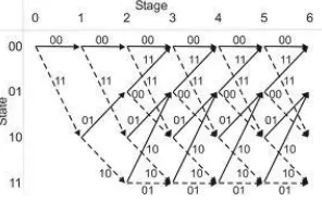
A path metric unit (PMU) summarizes branch metrics to get metrics for 2k-1 paths, where K is the constraint length of the code, one of which can eventually be chosen as optimal. Every clock it makes 2k-1 decisions, throwing off wittingly non-optimal paths. The results of these decisions are written to the memory of a trace-back unit (TBU). The core elements of a PMU are ACS (Add-Compare-Select) units. The way in which they are connected between themselves is defined by a specific code's trellis diagram (Fig 4). Since branch metrics are always , there must be an additional circuit preventing metric counters from overflow (it isn't shown on the image). An alternate method that eliminates the need to monitor the path metric growth is to allow the path metrics to "roll over", to use this method it is necessary to make sure the path metric accumulators contain enough bits to prevent the "best" and "worst" values from coming within 2(n-1) of each other. Trace-back unit (TBU) restores an (almost) maximum-likelihood path from the decisions made by PMU. Since it does it in inverse direction, a Viterbi decoder comprises a FILO (first-in-last-out) buffer to reconstruct a correct order. (A brief description is presented in this paper; more information can be seen in [10]). The allowable state transitions are represented by a trellis diagram. A trellis diagram for a K = 3, 1/3-rate encoder can be shown in Figure 4.
Fig 4: Trellis diagram for rate 1/3, K = 3 convolutional
In this example, the constraint length is three and the number of possible states is 2K–1 = 22 = 4 [10].
3.3 Serial VA Implementation
In this work, three types of serial VA programs have been studied and built, one with MATLAB code and the others with C++ code.
The VA serial algorithm steps are as follows: 1. Build the convolutional encoder. 2. Build the Viterbi decoder.
Through this work, the convolutional encoder (Fig 2) have been build. The input of the encoder will be entered as one bit at each time (k=1) which means that there is two probability of input data stream (0 or 1), (n=2) will gives two output bits at a time. This process will continue until all bits of the data stream vector completely finished. The two output bits (G1,
G2) calculated according to the following polynomials (g1 and
g2 are the content of the shift register):
2 1
1 1 g g
G ……… (1)
2
2
1
g
G
………. (2)The Viterbi algorithm involves calculating the hamming distance between the received bits, at time ti, and all the trellis
path segments (bits) entering each state at time ti. The Viterbi
algorithm removes from consideration those trellis paths that are not possible candidates for the maximum likelihood choice [11]. The flowchart of this algorithm is shown in Fig 5 and Fig 6 (a, b and c).
[image:2.595.93.241.641.734.2]Start
Generate {d} bits and store
them in a vector called data with any
random length
Load all the contents of the shift register with zero
(reset all contents)
I = 0
Insert the vector element
data[i] to the shift register
Compute the two output bits using eq.(1)and(2) and
store them in the new
vector called datco
I = I + 1
I>2*d
End Shift each stage to
its right neighbor
[image:3.595.332.541.72.467.2]Yes No
Fig 5: Flow Chart of convolutional encoder.
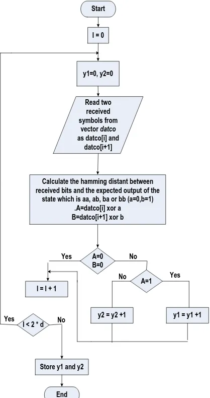
Start
Read two received symbols from
vector datco
as datco[i] and datco[i+1]
Calculate the hamming distant between received bits and the expected output of the
state which is aa, ab, ba or bb (a=0,b=1) .A=datco[i] xor a
B=datco[i+1] xor b I = 0
y1=0, y2=0
A=0 B=0
A=1
y1 = y1 +1 y2 = y2 +1
I = I + 1
I < 2 * d
Store y1 and y2
End Yes
Yes
Yes No
No
No
Start
Prepare two branch metric with zero value , r1=0 , r2=0
Add the branch metric with previous cost Newcost1 = r1+ y1 , newcost2 = r2 + y2
I = 0
Compare the two new cost min.cost = newcost1- newcost2
Min.cost < 0
min.cost=newcost2 Update the branch metric
r2=min.cost1
min.cost=newcost1 Update the branch metric
r1=newcost2
Record the decoded bit in vector called outputdetect as (0 or 1) according to state number
I = I + 1
I < 2 * d
End
Yes
Yes No
No
[image:4.595.54.279.68.458.2]Fig 6:(b) PMU Unit.
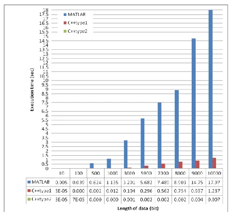
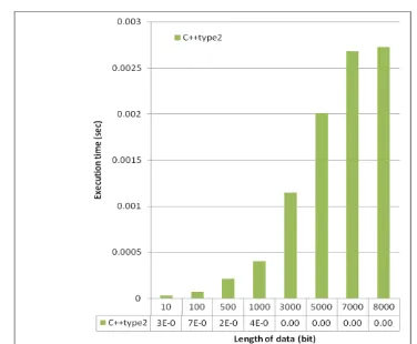
Table 1. Execution time in seconds for various lengths of input data
Length of data (bit)
MATLAB C++ type 1 C++ type 2
10 0.005448 0.000032 0.000034
011 0.039038 0.000163 0.000073
011 0.624054 0.002757 0.000214
0111 1.135896 0.012674 0.000406
0111 3.201251 0.104847 0.001148
0111 5.682160 0.296681 0.002008
0111 7.489519 0.562506 0.002683
0111 8.903280 0.754925 0.002725
0111 14.757222 0.936984 0.004870 01111 17.976502 1.237444 0.007100
Start
Read the four min.cost from all four state
I = 0
Searching the min from these four cost
I = I + 1
I > 4
Select the vector with min. cost as the transmitted data stream
End Yes
No
Fig 6: (c) Trace-Back Unit (TBU)
[image:4.595.362.487.69.415.2] [image:4.595.312.543.479.693.2]Fig 8: Execution time in seconds for various lengths of input data (type 2)
4. PARALLEL COMPUTING
A parallel computer is a set of processors that are able to work cooperatively to solve a computational problem. This definition is broad enough to include parallel supercomputers that have hundreds or thousands of processors, networks of workstations, multiple-processor workstations, and embedded systems [12].
Parallel processing is an efficient form of information processing which emphasizes the exploitation of concurrent events in the computing process. Parallel events may occur in multiple resources during the same time interval, simultaneous events may occur at the same time instant, and pipelined events may occur in overlapped time span [13].
Parallel computer systems are broadly classified into two main models based on Flynn’s specifications: single-instruction data (SIMD) machines and multiple-instruction multiple-data (MIMD) machines [14].
The motivations for parallel processing can be summarized as follows [15]:
1. Higher speed, or solving problems faster. This is important when applications have "hard" or "soft" deadlines. For example, there is at most a few hours of computation time to do 24-hour weather forecasting or to produce timely tornado warnings.
2. Higher throughput, or solving more instances of given problems. This is important when many similar tasks must be performed.
4.1 Parallelism Type Classification
Computer organizations are characterized by the multiplicity of the hardware provided to service the instruction and data streams. Listed below are Flynn’s four machine organizations [16]:
SISD – Single Instruction stream / Single Data stream. SIMD – Single Instruction stream / Multiple Data stream. MISD – Multiple Instruction stream / Single Data stream.
MIMD – Multiple Instruction stream / Multiple Data stream.
4.2 Parallel VA Implementation
The parallel distribution of Viterbi Algorithm tasks are illustrated using the following methods:
1. Distributing the states of trills diagram between numbers of computers in a local area network (LAN) as a multi-computers system.
2. Decomposing the length of received data stream to more than one computer using the same network (LAN).
4.2.1 Parallel State Viterbi Decoder
The parallel VA algorithm steps are as follows: 1. Initialization: Defining variables.2. Encoder process: Generating the data vector with any random length, and encoding it using convolutional process.
3. MPI Initialization: MPI initialization is done using MPI_Init function (MPI programing).
4. Decomposed task: Distributing the computational amount between number of processors or computers, in this work each state in the trills diagram have been built by a processor unit.
5. MPI Finalize: MPI_Finalize function (MPI programing) is used to terminate MPI package.
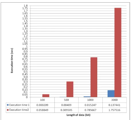
The computations in a state are dependent on the previous state. So there is data movements between the states, these movements will add considerable time to the execution time. The serial Viterbi decoder type 1 have been implemented in typical PC computer and the results are in Table 2 and can be shown in Fig 9. The parallel implementation for this algorithm is tested on a LAN network which has a speed of 100 Mb/s with four typical PC computers. From Fig 9, it can be concluded that there is no benefit from the use of this parallelization method since the delay is very large in compared with the serial one.
Table 2. Execution time for type 1 Viterbi Decoder
Length of data (bit)
Execution time1(sec)
(serial)
Execution time2(sec)
(parallel)
100 0.000209 0.058849
500 0.004090 0.309505
1000 0.015247 0.785667
3000 0.137441 1.757516
[image:5.595.353.504.426.568.2]
Fig 9: Execution time for type 1 Viterbi Decoder
Start
I = 0
Each computer will receive the same costs and vectors from specified states
of the previous cycle (ti-1).
I = I + 1
I > 2 * d
Send the final result to computer 1.
End Yes No
Run branch metric and path metric operations in the current cycle (ti) using
that received symbols.
Select the vector with min. cost as the transmitted data stream
Fig 10: Flow chart of parallel states VA
4.2.2 Block Based Parallel Viterbi
[image:6.595.322.542.233.311.2]Better performance can be achieved by decomposing the data stream into blocks of length N which can be processed independently in parallel using K Viterbi processors (VP). Processing K blocks in parallel causes an increase in the throughput (speedup equal to K). Each processor will take a part of the data received, and apply the Viterbi Algorithm on it. In the serial Viterbi decoder program, one processor will work for thousands cycles (length of received data) to reconstruct the original data, but in the proposed system, these cycles have been divided between more than one processor or computer, so that the execution time of the program decreases with increasing the number of computers until critical range. Figure 11 shows the mechanism for this parallelism.
.
Data Stream
Data Blocks
[image:6.595.70.268.306.748.2]VP1 VP2 VP3 VP4
Fig 11: Generic block based parallel Viterbi.
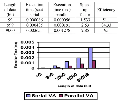
The advantages of this method of parallelism is appears when the receiver have been received the entire frame of the transmitted data stream before processing them. Different number of computers can be used. Ideally, if two computers work in parallel, the execution time will be reduced to half the time of serial program, then again; in the practical case there is a small amount of time would be lost for input and or output data between the computers. For huge data, this time may be neglected compared with the computation time. This parallel program also implemented in one computer as multi-processes. In this part of the work, serial Viterbi decoder type 2 (which has execution time less than Viterbi decoder type 1) will be considered in the result of serial and parallel programs. The serial Viterbi decoder type 2 was implemented on PC computer type LGA with Celeron®, CPU and RAM of 1GB and the results can be shown in Table 3. The speedup and efficiency could be computed using equation 3 and 4 respectively.
p s
T
T
Speedup
………. (3)where Ts : Time to perform a task by a single computer.
Tp : Time to perform a task by multicomputer.
n
Speedup
Efficiency
……. (4)
Table 3. The execution time, speedup and efficiency of the Viterbi decoder type 2 (two computers)
Length of data (bit)
Execution time(sec) (serial) ,
Ts
Execution time (sec)
(two computers),
Tp
Speed-up factor
Ts / Tp
Efficiency
From figure 11 one can conclude that in the case of using two computers execution time will be reduced approximately by half and not exactly to half due to communication overhead.
0 0.001 0.002 0.003 0.004 0.005
100 1000 3000 6000 8000 1000
0
Length of data (bit)
E x e c ut ion Ti m e ( s e c )
[image:7.595.306.552.99.384.2]Serial VA Parallel VA
Figure 11: The execution time of the Viterbi decoder type 2 (two computers)
The delay have been evaluated when the proposed algorithm is tested on a 3 PC and 4 PC (table 4 and 5). Figure 12 and 13 shows the result when the number of computers is three and four respectively. The execution time relative to the communication time have become greater with four computers.
[image:7.595.65.280.111.243.2]The results show that the speedup factor and efficiency differ from system to another. In addition, it changes with changing the message length. Ideal speedup is equal to the number of computers. The proposed system have an overhead due to the communications. Figure 14 and 15 shows the comparisons between these systems in terms of a speedup and efficiency respectively.
Table 4. The execution time, speedup and efficiency of the Viterbi decoder type 2 (three computers)
Length of data (bit) Execution time (sec) serial Execution time (sec) parallel Speed up factor Efficiency
99 0.000086 0.000056 1.533 51.1 999 0.000485 0.000191 2.53 84.33
9000 0.003655 0.001278 2.85 95
0 0.001 0.002 0.003 0.004 0.005
99 999
3000 60009999 9
Length of data (bit)
Ex ec ut ion Tim e (s ec )
Serial VA Parallel VA
[image:7.595.363.496.418.531.2]Fig 12: The execution time of the Viterbi decoder type 2 (three computers)
Table 5. The execution time, speedup and efficiency of the Viterbi decoder type 2 (four computers)
Length of data (bit) Execution time (sec) serial Execution time (sec) parallel Speed up factor Efficiency
100 0.000086 0.000044 1.954 48.86 1000 0.000485 0.000214 2.266 56.65 3000 0.001393 0.000597 2.333 58.333
6000 0.002737 0.001711 1.6 40
8000 0.003655 0.001578 2.316 57.91 10000 0.004505 0.001949 2.311 57.79
0 0.001 0.002 0.003 0.004 0.005
100 1000 3000 6000 8000 1000
0
Length of data (bit)
E x e c ut ion Ti m e ( s e c )
[image:7.595.45.289.452.661.2]Serial VA Parallel VA
Fig 13: The execution time of the Viterbi decoder type 2 (four computers) 0 0.5 1 1.5 2 2.5 3
2 3 4
Number of computers
Sp e e d u p fa c to r
Fig 14: Speedup for the proposed system.
0 0.1 0.2 0.3 0.4 0.5 0.6 0.7 0.8 0.9 1
2 3 4
Number of comuters
Effi c ie n c y
Fig 15: Efficiency for the proposed system.
4: CONCLUSIONS
[image:7.595.370.490.572.675.2]There are VA implementations on microprocessors, CMOS technology, etc. The design of a four state convolutional encoder and Viterbi decoder has been studied and implemented using MATLAB code and C++ code with the long truncation depth and with small truncation depth (recursive method). It is found that the MATLAB code delay is greater than the C++ code delay. In addition, the delay with long truncation depth is greater than with small truncation depth. For trills diagram of Viterbi decoder, a greatly computations has been required in the decoding process. Searching the maximum likelihood sequence path is a time consuming effort. This time is grown exponentially with increasing the complexity of the Viterbi trills diagram. So, it is proposed to parallelize the Viterbi algorithm to reduce this time. There are many available choices for parallelization. In this paper, message passing interface (MPI) with dual core personal computer (PC) and then with cluster is selected as the environments to parallelize VA. The Viterbi algorithm is parallelized by distributing the states on the cluster and by using block based technique. Performances of these parallel VA codes are tested on different number of computers. It is found that the parallel Viterbi code when the states have been distributed on a number of computers provide poor performance; due to the communication overhead. So; it will be suggested that to replace the multicomputer system (LAN with 100Mbps) with multiprocessor system (its speed tenth of Gbps). Better performance have been obtained with block based parallelism technique. Block based parallelism can reach a maximum efficiency of 94.25 % and speed-up of 1.88497 when 2 PCs are used on a cluster with message length of 3000 bits. On 3 PCs, maximum efficiency of 95% and speedup of 2.85 have been obtained with message length of 9000 bits. However; on 4 PCs; the system reaches maximum efficiency of 58.333, maximum speed-up of 2.33 with message length of 3000 bits.
The results show that the speedup factor and efficiency differ from system to another. In addition, it changes with changing the message length. It is concluded that the parallelization of Viterbi algorithm is successful. On the other hand the efficiency of the proposed systems is different.
5. REFERENCES
[1] Derwood, 2002. A Tutorial on Convolutional Coding with Viterbi Decoding.
[2] T. Oberg, 2001. Modulation, Detection and Coding.
[3] Yanyan1, X. and Dianren1 “The Design of Efficient Viterbi Decoder and Realization by FPGA” Modern Applied Science; Vol. 6, No. 11; 2012.
[4] Bocharova, H., Student Member, IEEE, Johannesson, Life Fellow, IEEE, and Kudryashov “A Closed Form Expression for the Exact Bit Error Probability for Viterbi Decoding of Convolutional Codes”. Copyright © 2012 IEEE.
[5] Suresh, R., Bala. “Performance Analysis of Convolutional Encoder and Viterbi Decoder Using FPGA”. International Journal of Engineering and Innovative Technology (IJEIT) Volume 2, Issue 6, December 2012.
[6]
Laddha, V. “Implementation of Adaptive Viterbi Decoder through FPGA”. IJESAT | Nov-Dec 2012
[7] Nayel Al-Zubi Pipelined Viterbi Decoder Using FPGA Research Journal of Applied Sciences, Engineering and Technologies, 2013 (Vol. 5, Issue: 04).
[8] J. Tuominen and J. Plosila, "Asynchronous Viterbi Decoder in Action Systems ", TUCS Technical Report, No 710, 2005.
[9] John Proakis, 1989. Digital Communications.
[10] H. Hendrix, "Viterbi Decoding Techniques for the TMS320C54x DSP Generation ", TEXAS Application Report, SPRA071A - January 2002.
[11] Y. E. MAJEED, " Detection Methods for GSM/EDGE Mobile Communication System ", Ph.D. Thesis, University of Baghdad, 2007.
[12] I. Foster, 1995. Argonne National Laboratory, Designing and Building Parallel Programs: Concepts and Tools for Parallel Software Engineering.
[13] K. Hwang and B., 1988. Computer Architecture and Parallel Processing.
[14] A. Y. Zomaya, 2006. Parallel Computing for Bioinformatics and Computational Biology.
[15] B. Parhami, 2002. Introduction to Parallel Processing Algorithms and Architectures.