Munich Personal RePEc Archive
Bayesian VAR Models for Forecasting
Irish Inflation
Kenny, Geoff and Meyler, Aidan and Quinn, Terry
Central Bank of Ireland and Financial Services Authority of Ireland
December 1998
Online at
https://mpra.ub.uni-muenchen.de/11360/
Technical Paper
4/RT/98
December 1998
Bayesian VAR Models for Forecasting Irish Inflation
By
Geoff Kenny*, Aidan Meyler and Terry Quinn
Bayesian VAR Models for Forecasting Irish Inflation
Abstract
In this paper we focus on the development of multiple time series models for forecasting Irish Inflation. The Bayesian approach to the estimation of vector autoregressive (VAR) models is employed. This allows the estimated models combine the evidence in the data with any prior information which may also be available. A large selection of inflation indicators are assessed as potential candidates for inclusion in a VAR. The results confirm the significant improvement in forecasting performance which can be obtained by the use of Bayesian techniques. In general, however, forecasts of inflation contain a high degree of uncertainty. The results are also consistent with previous research in the Central Bank of Ireland which stresses a strong role for the exchange rate and foreign prices as a determinant of Irish prices.
1. Introduction
The primary focus of monetary policy, both in Ireland and elsewhere, has traditionally
been the maintenance of a low and stable rate of aggregate price inflation as defined by
commonly accepted measures such as the consumer price index. The underlying
justification for this objective is the widespread consensus supported by numerous
economic studies that inflation is costly insofar as it undermines real,
wealth-enhancing, economic activity.1 If anything, this consensus is probably stronger today
than it ever has been in the past. Indeed, it could be argued that much of the
improvement in Irish living standards which has taken place over the last ten years
would not have been achieved without the establishment of a credible low inflation
environment.
From the beginning of 1999, the Irish economy confronts a new environment in which
monetary policy will be set by the Governing Council of the European Central Bank
(ECB). The Irish decision to participate in European Economic and Monetary Union
(EMU) represents an attempt to secure this new era of price stability once and for all
since the associated fixing of exchange rates removes much of the nominal exchange
rate variation which has been a primary source of price instability in the Irish economy.
Reflecting the broad consensus noted above, the ECB is committed to a monetary
eleven countries which comprise the euro area. In this new setting, forecasts of
inflation for the euro area will represent a key ingredient in designing policies which
are geared toward the achievement of price stability. Hence, even though Ireland’s
weight in the overall euro area price index is relatively small, forecasts of Irish inflation
will continue to be required. Moreover, such forecasts should be optimal in the sense
that they make use of all relevant indicators and weight them correctly according to
their reliability as predictors of future price developments.
Apart from its role as an input into monetary policy, however, forecasts of Irish
inflation are likely to have a continued - or perhaps even greater - role in other areas of
economic policy-making. In particular, it has been argued that the sacrifice of
monetary autonomy which results from Irish participation in EMU has increased the
need to consider fiscal policy as a counter-cyclical demand management tool (or at
least fiscal policy should not adopt a pro-cyclical stance). Arguably, therefore, the
inflation forecast should be given greater weight in the formulation of fiscal policy in
Ireland than has been the case in the past. Furthermore, it is clearly the case that
notwithstanding the common money which is shared by each participant in EMU,
inflation differentials are likely to arise between member states.2 On the one hand, such
differentials may be warranted in the presence of productivity differentials between the
traded and non-traded sectors of individual economies. However, should they persist,
such differentials may also be a sign of economic inefficiencies which could undermine
a countries competitiveness. With nominal exchange rates fixed vis-à-vis other EMU
participants, the forecast of Irish inflation is therefore essentially a forecast of the likely
evolution of Irish competitiveness within the euro area. As such, it is likely to have a
stronger and perhaps more transparent impact on the wage-bargaining process.
Most previous Central Bank studies of Irish inflation have focused on attempting to
impose or test economic theories such as the purchasing power parity doctrine and not
1Two recent studies are Feldstein (1996) and Dotsey and Ireland (1996). Both of these papers argue
on forecasting per se. Since forecasting is in fact one of the most important goals of empirical analysis, this represents a significant shortcoming. In this paper we
undertake an analysis of Irish inflation which is not geared toward confirming or
refuting any particular economic theory. Instead, we focus on the development of a
multiple time series model purely for forecasting purposes.3 The analysis is therefore
data-intensive insofar as it assesses a host of indicator variables as potential candidates
for inclusion in a vector autoregressive model of Irish prices. In addition, unlike
previous studies, we focus on the Harmonised Index of Consumer Prices (HICP) as
the relevant measure of inflation given its policy relevance in the new environment
associated with EMU.
Following Doan, Litterman and Sims (1984), the Bayesian approach to the estimation
of vector autoregressions (VARs) is employed.4 The use of VARs in empirical
macroeconomics is a subject of some dispute. Macroeconomic forecasting models
have traditionally been formulated as simultaneous equation structural models.
However, for a variety of reasons - such as the inexact manner in which certain
variables are excluded from the model’s equations and the need to include future
values of exogenous variables - structural models have proved unreliable for
forecasting. 5 VARs offer an alternative to structural macroeconomic models for
forecasting purposes. In contrast to structural models, a vector autoregressive model is
a set of dynamic linear equations in which each variable is determined by every other
variable in the model. However, VARs have also been criticised insofar as they lack
strong theoretical justification over and above the use of theory as a guide in deciding
2 For a recent discussion and empirical analysis of this issue see Alberola and Tyrvainen (1998).
3 In a complementary paper, Meyler, Kenny and Quinn (1998) focus on forecasting Irish Inflation
using ARIMA time series models.
4 An earlier study which uses the astructural VAR methodology in an analysis of Irish prices is
Howlett and McGettigan (1995). This paper does not however use the Bayesian approach to parameter estimation.
5 The evidence in Stockton and Glassman (1987) shows that a simple ARIMA model for forecasting
which variables to include in the analysis. 6 Doan, Litterman and Sims (1984) in an
attempt to improve the forecasting performance of unrestricted VARs suggested that
they could be estimated using Bayesian techniques which take account of any prior
information which may be available to the modeller. It is this Bayesian approach to
parameter estimation in vector autoregressions which is employed in this study.
The layout of the paper is as follows. Section 2 reviews the Bayesian approach to the
estimation of the parameters in vector autoregressions. With a view to deciding which
variables to include in our VARs, Section 3 assesses the relative strength and
significance of various inflation indicators in forecasting Irish inflation at different
horizons. Section 4 compares and contrasts the forecasting performance of three
alternative Bayesian VARs. Finally, Section 5 summarises and concludes.
2. Bayesian Vector Autoregressions - An Overview
There is a growing body of empirical evidence which suggests that Bayesian VARs
produce forecasts which set a high standard of comparison for most alternative
methods such as univariate time series models or large-scale macro-models.7 This is
particularly true in the case of real macroeconomic variables such as output, the
unemployment rate and the balance of payments and particularly at long horizons.8 In
the area of inflation forecasting, however, the performance of BVAR models has been
somewhat less impressive. The BVAR model reviewed in Litterman (1986), for
example, produced inflation forecast errors which are on average twice the size of the
forecast errors of conventional or professional economic forecasters.9 Among other
recent studies which document the relatively poor performance of the inflation
6 Canova (1993), section 6, describes various other critiques of the VAR methodology.
7 Early evidence is contained in Doan, Litterman and Sims (1984), Todd(1984), Litterman
(1984,1986) and McNees(1986). More recent applications of the BVAR methodology include Alvarez, Ballabriga and Jareno (1998), Dua and Ray (1995) and Webb (1995).
8 See, for example, McNees (1986).
forecasts produced by BVAR models are Webb (1995) and also Zarnowits and Braun
(1991). In the former study, for example, the forecasts of a Bayesian VAR are either
worse than - or at least not significantly better than - a “no-change” forecast at all
horizons examined. Against this, however, Artis and Zhang (1990) use the Bayesian
approach in the estimation of VARs for the G7 summit group of countries. For most
countries examined, the Bayesian VAR predictions of inflation are as accurate as the
forecasts of output and the balance of payments. In addition, the authors find that the
BVAR models “set tough standards of comparison for forecasts produced by more
traditional methods” (including the forecasts produced by the IMF in its World Economic Outlook). More recently, Alvarez, Ballabriga and Jareno (1998) have estimated a BVAR model for the Spanish economy and evaluated its forecasting
performance relative to an unrestricted VAR and also a Bayesian univariate
autoregression. These authors find that “it is in the forecasting of the price variable
that the superiority of the BVAR model over the other models becomes clear and the
differences are quite important” (p. 386). In light of such evidence, the construction
and evaluation of Bayesian VARs for inflation forecasting purposes in Ireland is a
potentially worthwhile undertaking. Before doing so, however, we review some of the
details involved in the application of Bayesian techniques to modelling economic time
series and to vector autoregressions in particular.
2.1 Bayesian Statistics
The Bayesian approach to statistics provides a general method for combining a
modeller’s beliefs with the evidence contained in the data. In contrast to the classical
approach to estimating a set of parameters, Bayesian statistics presupposes a set of
prior probabilities about the underlying parameters to be estimated. For example one
might have a strong prior that the first autoregressive coefficient in an AR(p) model for the exchange rate is equal to unity and that all other coefficients are zero. Such a prior
would be consistent with the view that the exchange rate follows a random walk or
the parameters of an AR(p) model will revise this prior view in the light of the empirical evidence contained in a time series of foreign exchange data. A prior
hypothesis about a particular parameter value can thus be confirmed by any
observation which is likely given the truth of the prior hypothesis (or unlikely given its
falsehood). This contrasts significantly with classical approaches to parameter
estimation such as the method of maximum likelihood where one chooses as point
estimates values such that the likelihood of obtaining the actual sample of data is
maximised regardless of any prior probabilities which are or could be assigned to the
parameters.
More formally, in the Bayesian approach, the nonsample prior information about the
set of parameters which is to be estimated,
θ
= {θ1, θ2, θ3, . , . , θn}, is taken to beavailable in the form of a prior probability density function, g(
θ
). Prior probabilitystatements that one might wish to make about
θ
can be expressed as integrals of theprior probability density function. Consider, for example, the AR(p) model for the
exchange rate (St) which can be expressed as equation (2.1) below,
St = θ1 St-1 + θ2 St-2 + . . . + θp St-p + εt
(2.1)
where εt is a white noise disturbance term. In this case the set of parameters to be
estimated is comprised of the p autoregressive coefficients,
θ
= { θ1, θ2, θ3, . . ., θp).Prior statements can be expressed mathematically using the set of univariate prior
density functions g(θ1), g(θ1), . . . , g(θp). The “random walk” prior which one might
unity whereas the means of all other autoregressive parameters of higher order than
one are zero. This prior view could be expressed as (2.2) below.
E[θ1] = θ1 g(θ1)dθ1 =1 −∞
∞
∫
E[θ2] = θ2 g(θ2)dθ2 =0 −∞
∞
∫
. . . .
. . . .
. . . .
E[θp] = θp g(θp)dθp =
−∞ ∞
∫
0(2.2)
where E[ ] denotes the expectations operator. One notable feature of the priors
contained in (2.2) is that such statements can be easily modified to reflect the degree of
confidence that the empirical modeller has that the prior is true. For example, one
might believe that coefficients on higher order lags are more likely to be zero than
lower order lags. This tightening of the prior for higher lags could be achieved by
letting the prior variance decrease with increasing lag length.10 The objective of
Bayesian estimation is however to produce coefficient estimates which combine the
evidence from the sample of data with the information contained in the prior. The
information contained in the sample of data is summarised in the sample probability
density function, g(St|
θ
), which can be viewed as the density of the random variable
St conditional on the value taken by the parameters in θ. The two types of information
- prior and sample - are combined into a posterior density function g (θ| St ) using
Bayes’ Theorem, i.e.
g
S
g S
g
g S
t
t t
( | )
( | ) ( )
( )
θ
=
θ
θ
(2.3)
where g(St) is the unconditional density of St which, for a given sample of data, is a
normalisation which ensures that g (θ | St ) is a well behaved probability density
function. 11 The posterior density function contains all the available information about
θ and from it point estimators can be derived. The mean of the posterior distribution
is, for example, often taken as a point estimate for θ.
2.2 Bayesian Vector Autoregressions
In forecasting economic time series, the Bayesian approach has most often been
applied to multivariate vector autoregressions rather than to the univariate models such
as the AR(p) model mentioned above. A Bayesian approach to vector autoregressions
has in particular been put forward by Doan, Litterman and Sims (1984). The priors
suggested in these two papers, usually referred to as the Minnesota or Litterman
11 Bayes’s formula is often viewed as being relevant in situations where the outcomes of random
priors, were suggested for an n-dimensional VAR of non-stationary variables.12
Consider the n variable vector autoregression of order p, VAR(p), given by (2.4) below,
y
t = Γ1 yt-1 + ... + Γpy
t-p +µ
+ε
t(2.4)
where yt is an (n x 1) vector of non-stationary time series, µ is an (n x 1) vector of
constants coefficients and εt is an n x 1 vector of error terms. Γ1 through Γp represent
(n x n) matrices of parameters to be estimated.13 The VAR(p) is therefore simply a set
of equations in which each variable depends on a constant and lags 1 through p of all n
variables in the system. Each equation in the VAR contains exactly the same number
of explanatory variables and can be estimated by ordinary least squares (OLS).
However, the above system has exactly n + pn2 parameters to be estimated. Not surprisingly therefore empirical results from the estimation of unrestricted VARs often
yield coefficient estimates which are imprecise and not significantly different from zero.
This problem of over-parameterisation is particularly acute in the small sample sizes
which are generally available to macroeconomic forecasters. Indeed several studies
12 Hence when the VAR contains only stationary I(0) variables, or when it combines both I(1) and I(0)
variables it is necessary to amend the original Minnesota prior somewhat. See Lutkepohl (1991), Ch. 5., for a modified version of the Minnesota prior for an n-dimensional VAR of stationary time series.
13 The original contribution of Doan, Litterman and Sims (1984) allowed time-variation in these
have been published which show that unrestricted VAR models produce poor
out-of-sample forecasts for macroeconomic variables such as inflation and output.14
To counteract the problem of over-parameterisation, Doan, Litterman and Sims (1984)
suggest the application of Bayesian procedures in the estimation of the parameters of
the system described by (2.4) above. The original Litterman or Minnesota prior was
based on the idea that each series is best described as a random walk around an
unknown deterministic component. Hence the prior distribution is centred around the
random walk specification for variable n given by (2.5) below.
y
n,t = µn + yn,t-1 +ε
n,t(2.5)
According to this specification, the mean of the prior distributions on the first lag of
variable n in the equation for variable n is equal to unity. The mean of the prior distribution on all other coefficients is equal to zero. Of course, if the data suggest
that there are strong effects from lags other than the first own lag or from the lags of
all the other variables in the model this will be reflected in the parameter estimates. No
prior information is assumed to be known about the prior mean on the deterministic
components.15 Furthermore, the prior distributions on all the parameters Γ
1 through Γp are assumed to be independent normal. Hence, once the means have been specified,
the only other prior input is some estimate of the dispersion about the prior mean. As
14 In Section 4 of the paper, the inflation forecasting performance of a variety of unrestricted VAR is
compared with that of the Bayesian approach.
described in Litterman (1986), the standard error on the coefficient estimate for lag l of variable j in equation i is given by a standard deviation function of the form S(i, j, l) given by equation (2.6) below.
[
]
S i j l g l f i j s s
i j
( , , )= γ ( ) ( , )
(2.6)
where
f (i, j) = 1 if i = j and wij otherwise
(2.7)
The “hyperparameter” γ and functions g(l) and f(i, j) determine the tightness or weight attaching to the prior in (2.5) above. Given the functional specifications of g(l) and f(i, j), γ can simply be interpreted as the standard deviation on the first own lag.16 It is also
often termed the “overall tightness” of the prior. The function g(l) determines the tightness on lag one relative to lag l. The tightness around the prior mean is normally assumed to increase with increasing lag length. This is achieved by allowing g(l) decay harmonically with decay factor d, i.e. g(l) = l-d.17 The tightness of the prior on variable
16 If for example γ = 0.5, the standard deviation on the first own lag in each equation of the VAR
would be equal to 0.5 because g(1) = f(1, 1)=s1 /s1 =1.
17 Increasing d is, therefore, a way of tightening the prior with increasing lag length. With d equal to
j relative to variable i in the equation for variable i is determined by the function f(i, j);
this can be the same across all equations in which case wijis equal to a constant (w) and the prior is said to be symmetric. Alternatively, the tightness of the prior for variable j
relative to variable i (in the equation for variable i) can vary depending upon the particular equation and/or variable in question (this is known as a general prior). However, the flexibility inherent in the specification of a general prior may not always
be desirable. On the one hand, as argued by Doan (1990), it simply transfers the
problem of over-parameterisation to one of having to estimate or search over too many
hyperparameters. However, in a situation where the analyst has strong prior views
that one of the variables is exogenous, the general prior may improve forecasting
performance.18 In particular, the equations for exogenous variables may best be
specified as univariate autoregressions with no feedback from the other variables in the
system. This can be achieved by setting very low values for the off-diagonal elements
in f(i, j) which correspond to that particular variable.
Finally, the multiplicative ratio si/sj in equation (2.6) reflects the fact that in general the
prior cannot be completely specified without reference to the data. In particular it
corrects for differences in the scale used in the measurement of each variables included
in the system. For example, how tight a standard deviation of 0.5 is on the lags of
prices in an equation for the interest rate will depend on whether the price index is
based to equal unity or 100 in the base period. Litterman (1986) argues that the scale
of the response of one variable to another is “a function of the relative size of
unexpected movements in the two variables rather than the relative sizes of their overall standard errors”. Hence, he suggests scaling the standard error on the prior by
the ratio of the standard deviations of the residuals (si) from a univariate
etc. An alternative is to use a geometric decay function. Doan (1990), however, suggests that this leads to too rapid a tightening of the prior as the lag length increases.
18 Such a situation is likely to arise particularly in BVARs for a small open economy such as Ireland.
autoregression for variable i to the standard deviation of the residuals (sj) from a
univariate autoregression for variable j (both with p lags).
2.3 Estimation
In estimating the parameters of the BVARs reported in this paper, Theil’s (1963)
mixed estimation technique is employed.19 Mixed estimation is a relatively simple and
intuitive means of combining sample information with stochastic prior information (for
a discussion see Davidson and McKinnon, 1993). Suppose that we have m priors which we wish to take account of in deriving Bayesian estimates of the parameters of a
VAR. The idea is to estimate a regression with N + m observations:N of them corresponding to the information in the sample and m of them corresponding to the restrictions. The m observations corresponding to the restrictions are weighted relative to the observations in the sample according to the degree of tightness in each
prior. As the amount of information in the prior tends toward zero, i.e. for an
extremely “diffuse” prior, the mixed estimators of the parameters of a BVAR tend
toward the OLS estimates of the parameters of an unrestricted VAR. Conversely,
when the priors are extremely informative or precise, the mixed estimators tend
toward a set of parameters which satisfy the prior restrictions.
3. Inflation Indicators
Before considering in detail the actual performance of a selection of BVAR models in
predicting future Irish inflation, it is necessary to first consider the issue of which
variables to include in the VAR specification. From an economic viewpoint, changes
in the level of aggregate prices are likely to emanate from a wide array of different
sources. There is therefore a very large class of different variables which may help to
predict the future evolution of inflation and there is a large measure of judgement
19 Hamilton (1994) discusses several alternative numerical approaches. For example, in large samples
needed in deciding which variables to consider a priori. Below, we examine the relevance of various indicators of Irish inflation. These include various domestic prices
series, monetary and financial variables, indicators of the level of activity or demand in
the domestic economy, foreign price variables and also various world commodity
prices. In addition, economic theory would suggest that different indicators will help
forecast inflation at different horizons. Hence, the usefulness of the above variables is
assessed for various forecast horizons (from 1 quarter to 3-4 years ahead). In order to
do this we follow Cecchetti (1995) and estimate the following regression (3.1),
πt+l, t+k = a(L) πt + b(L) Xt + εt(l, k)
(3.1)
where πt+l, t+k is inflation from t+l to t + k, πt is the rate of inflation from t-1 to t, Xt is
the indicator variable to be tested, a(L) and b(L) are lag polynomials of order 6 and εt
is a stationary moving average error process of order k-1. The equation is estimated over the period since Ireland joined the European Monetary System to the present
(1979:1 - 1998:1).
As discussed above, the selection of the variables could not be exhaustive and
necessarily involves judgement. We chose a host of domestic price series such as
wages and manufacturing output prices, domestic monetary aggregates such as credit
and the broad money stock, the nominal effective exchange rate, indicators of the level
of domestic demand such as retails sales and import volumes and also two alternative
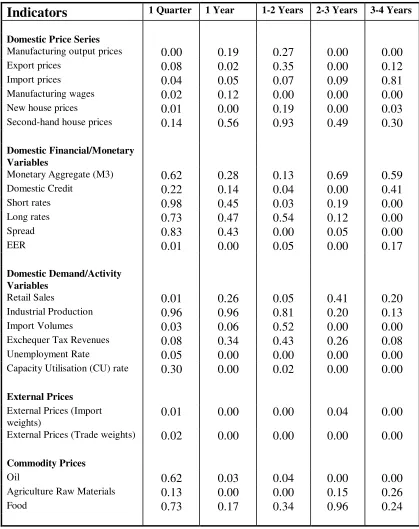
Table 3.1 Wald Test (P-Values) for the Significance of Various Inflation Indicators Sample: 1979:1-1998:1
Indicators
1 Quarter 1 Year 1-2 Years 2-3 Years 3-4 Years Domestic Price SeriesManufacturing output prices 0.00 0.19 0.27 0.00 0.00
Export prices 0.08 0.02 0.35 0.00 0.12
Import prices 0.04 0.05 0.07 0.09 0.81
Manufacturing wages 0.02 0.12 0.00 0.00 0.00
New house prices 0.01 0.00 0.19 0.00 0.03
Second-hand house prices 0.14 0.56 0.93 0.49 0.30
Domestic Financial/Monetary Variables
Monetary Aggregate (M3) 0.62 0.28 0.13 0.69 0.59
Domestic Credit 0.22 0.14 0.04 0.00 0.41
Short rates 0.98 0.45 0.03 0.19 0.00
Long rates 0.73 0.47 0.54 0.12 0.00
Spread 0.83 0.43 0.00 0.05 0.00
EER 0.01 0.00 0.05 0.00 0.17
Domestic Demand/Activity Variables
Retail Sales 0.01 0.26 0.05 0.41 0.20
Industrial Production 0.96 0.96 0.81 0.20 0.13
Import Volumes 0.03 0.06 0.52 0.00 0.00
Exchequer Tax Revenues 0.08 0.34 0.43 0.26 0.08
Unemployment Rate 0.05 0.00 0.00 0.00 0.00
Capacity Utilisation (CU) rate 0.30 0.00 0.02 0.00 0.00
External Prices
External Prices (Import
weights) 0.01 0.00 0.00 0.04 0.00
External Prices (Trade weights) 0.02 0.00 0.00 0.00 0.00
Commodity Prices
Oil 0.62 0.03 0.04 0.00 0.00
Agriculture Raw Materials 0.13 0.00 0.00 0.15 0.26
list of all the variables considered is given in Table 3.1 and the data sources are
described in detail in Appendix II. Except for the interest rate variables, the
unemployment rate and the capacity utilisation rate, all the indicators were logged and
differenced once. Table 3.1 reports the results from the estimation of equation (3.1)
for 5 different horizons: 1 quarter ahead (l = 0, k = 1), 1 year ahead (l=0, k=4) , 1-2 years ahead (l=4, k=8), 2-3 years ahead (l=8, k = 12) and 3-4 years ahead (l=12, k= 16). As in Cecchetti (1995), the Table reports P-values for the Wald test that all the
elements of b(L) are zero simultaneously. This test statistic is computed using a
covariance matrix of the estimated coefficients which is robust to heteroscedasticity
and serial correlation up to a moving average of known order.20 In Table 3.1, a
P-value greater than 0.05 suggests that the null hypothesis that the indicator has no
predictive power is acceptable at the 5% level of significance. Alternatively, the null of
no predictive power is rejected for P-Values less than 0.05.
From the Table, it can be seen that the performance of various indicators does indeed
depend significantly on the horizon which is being examined. Among the domestic
“price” series, only second-hand house prices do not help predict future inflation at any
of the different horizons examined. Against this, manufacturing wages, new house
prices, manufacturing output prices, import prices and export prices would appear to
be significant at predicting future variation in consumer prices at various horizons from
one quarter up to four years out.
Among the domestic monetary/financial variables, domestic credit contains some
information at horizons between one and three years but the broad monetary aggregate
is insignificant at all horizons examined. This is somewhat consistent with previous
research in the Central Bank. Howlett and McGettigan (1995), for example, found
some role for credit - but none for broad money - as a predictor of inflation at
medium-to-long horizons. Both short and long-rates would appear to contain some information
20 The covariance matrix is calculated using the Newey and West (1987) estimator with lags equal to
- the latter, however, only at horizons of three-to-four years out. However, the slope
of the yield curve, as proxied by the spread of long over short rates, has some
predictive power at horizons above one year.21 Lastly, consistent with the small open
economy view of Irish price determination, the nominal effective exchange rate (EER)
is significant over all horizons from one quarter ahead up to three years. The finding
that it is not significant at the very long horizon (3-4 years) suggests that all the effects
on inflation of past changes in the EER have passed through within about three years.
Among the measures of demand or “activity” in the domestic economy only the
unemployment rate is significant over all horizons. Neither exchequer tax revenues nor
the industrial output variable are found to contain any explanatory power at the 5%
level. In contrast both import volumes and the capacity utilisation rate are somewhat
significant at short and long horizons. Again consistent with the small open economy
view, external prices - whether weighted according to imports or average trade (import
and export) weights - are highly significant over all horizons from a single quarter out.
Finally, of the three international commodity price series examined, only oil prices and
the price of agricultural raw materials are significant.
In assessing the evidence in Table 3.1, it must be noted that the Wald test described
above represents a first-pass attempt to filter out any variables which do not have
significant correlations with inflation at various horizons. Variables which fail such a
test are unlikely to make any significant contribution to improving forecasting accuracy
in a multiple time series model. However, should a particular variable have significant
explanatory power on the basis of the regression described by equation (3.1) this does
not mean that it will retain this relevance in a vector autoregressive model which
includes other relevant variables. Hence, variables which emerge as significant
predictors of inflation on the basis of (3.1) may not emerge as being relevant in a
vector autoregressive model. Finally, it should also be noted that the significance and
21 A previous study, McGettigan (1995) found very little - if any - information in the Irish term
strength of such inflation indicators is likely to change over time. Cecchetti (1995), for
example, found that when he divided his sample up into two distinct sub-samples,
variables which proved significant in certain periods lost their significance in
subsequent periods. This might reflect changes in the extent to which the monetary
authority reacts to such information and/or structural breaks in the economic regime.
As part of the preliminary assessment of various inflation indicators, we also undertook
an analysis of sub-sample regressions. While the results are not reported here, it was
found that many of the above indicators did not exhibit a high degree of temporal
stability in their relationship with inflation.
4. BVAR Forecasts of Irish Inflation: Empirical Results
In this section, we present an evaluation of the performance of various Bayesian vector
autoregressive models of Irish inflation. These models include all (or at least most) of
the variables which emerged as significant predictors of inflation on the basis of the
analysis in the previous section. As is quite evident from the discussion in section 4
above, there is considerable “flexibility” with regard to the exact choice of variables to
include in any model. Below, the basic model-building strategy, as well as the chosen
procedure for evaluating the alternative models is described briefly.
4.1 Modelling Strategy
On the basis of the indicator analysis in the preceding section it would seem reasonable
to at least examine the forecasting performance of the following three vector
autoregressive models:
BVAR1: A three variable Small Open Economy (SOE) model which includes the
foreign consumer prices (P*) and the nominal effective exchange rate (E). This VAR,
embodies the implicit - and perhaps naive - assumption that all goods and services in
the Irish economy are traded. However, there is a significant body of empirical
evidence which suggest that the purchasing power parity doctrine holds as a long-run
proposition for aggregate Irish prices. The above model can therefore be viewed as
an interesting baseline model against which the forecasting performance of two
augmented models can be compared.
BVAR2: An Augmented SOE model which extends the simple small open economy
model (BVAR1) to account for the interaction between wages, prices and domestic
demand. Previous studies which examine the relevance of wages in the Irish
inflationary process include Callan and Fitzgerald (1989) and also, more recently,
Kenny and McGettigan (1999). As discussed in the latter paper, the absence of a
completely fixed nominal exchange rate and the presence of non-traded goods means
that there will always be scope for domestic wage pressures to influence domestic
prices. Furthermore, even in the absence of any “deep” structural relationship between
wages and prices, wage data may still contain incremental information (over and above
that contained in external prices and the exchange) which may be useful for forecasting
purposes. Retail sales (RS) are chosen as the relevant proxy for domestic demand
pressures. From a theoretical point of view, even if one adopts a long-run PPP view of
the determinants of Irish inflation, domestic demand pressures may help explain some
of the short-term variation in the price level about its fundamental or equilibrium level.
The existence of non-traded goods also provides justification for explicit inclusion of a
demand pressure variable since firms in the non-traded sector are more likely to take
advantage of demand pressures by increasing their profit margins (i.e. raising prices )
in an economic upturn.
BVAR3: A Monetary Model which extends the small open economy model
(BVAR1) to account for a possible role for domestic credit (DC) and short-term
predictor of Irish inflation at horizons of one quarter ahead out to three years. From a
theoretical point of view, the inclusion of this variable can also be justified by reference
to the existence of non-traded goods.22 The inclusion of short-term nominal interest
rates is less justifiable on the basis of the evidence in Table (3.1). However, it did
appear to be a significant explanatory factor at the very long horizon (3-4 years) and
its inclusion allows us to explicitly compute forecasts which are conditional on an
assumed level of the nominal interest rate. Moreover, economic theory would also
suggest that the short-term interest rate would improve both the fit and out-of-sample
forecasting performance of the domestic credit equation in the VAR. Where domestic
credit creation helps predict future inflation, this may in turn help produce better
forecasts for consumer prices.
In any empirical application of the BVAR methodology, the issue of whether the
variables in the VAR should be in log levels or differenced must be addressed. For a
number of reasons, we favour models which are estimated in levels rather than in first
differences. Firstly, the Minnesota prior where the variable in question is posited as
following a random walk with drift, is generally applicable only to economic series in
levels (or log levels). Secondly, differencing discards long-run information in the data
which may be of use for forecasting. Finally, if the data in question are cointegrated in
levels, a VAR in first differences will be misspecified because it does not incorporate
adjustment to the long-run cointegrating relationship within the systems dynamics.
Engle and You (1987) demonstrate that in such situations either a vector error
correction model or a VAR in levels is a better alternative to a differenced model. In
the empirical application of the BVAR methodology below, the models are accordingly
estimated with all the variables expressed in log levels. However, we also compare the
forecasting performance of these Bayesian models with unrestricted VARs in both
levels and first differences.
22 See, for example, Blejer and Leiderman (1981) for an early model which posits an explicit role for
4.2 Forecast Performance and Evaluation
In terms of forecast performance summary statistics we report the root mean squared
error (RMSE) and also Theil’s U statistic which is the ratio of the RMSE of the
relevant model to the RMSE of a naive forecast which assumes no change in the
quarterly inflation rate over the forecast horizon. A U statistic greater than unity is an indication of a model which has very little reliability as a forecasting tool. Denoting
πi f
n
( ) as the models ith prediction for the rate of inflation n steps into the future and πi
a
as the corresponding actual inflation outturn which is subsequently realised, these
summary statistics are defined as:
Root Mean Squared Error
RMSE (n) = ( )T ( i ( ))n
a i
f i
T
−1
∑
π −π 2THEIL’S U Statistic
U(n) =
( ) ( ( )) ( ) ( ( )) T n T n i a i f i T i a i i T − − ∗ − −
∑
∑
1 2 1 2 π π π πwhere T is the number of forecasts computed and πi
∗(n) is the n-step ahead forecast
based on a naive model which assumes no change in the quarterly rate of inflation from
its current level. In calculating the above statistics a recursive or sequential regression
procedure was used to produce forecasts and compare these to actually observed
inflation outturns. This involved first estimating each of the VARs using data from
1979Q1 through to 1992Q1; this models was then used to compute forecasts from one
up to eight quarters ahead. Next, each models coefficient were
re-estimated using data covering 1979Q1-1992Q2 and forecasts were again computed for
inflation for up to eight quarters ahead. This procedure was then continued through to
the end of the sample (1998Q1). There were accordingly T = 24 forecasts upon which
the 1-step ahead forecast performance statistics were based and T = (24-n) forecasts upon which the n-step ahead forecast statistics were based. It is therefore important to note that the performance measures reported below are based on a relatively small
sample.
4.3 Choice of Hyperparameters
A key issue in the estimation of Bayesian VARs is the choice of hyperparameters
which determine overall tightness (γ), the tightness on the prior mean of zero on cross
lags in each equation (w) and the decay parameter (d). A complete search over all
possible hyperparameters is not justifiable insofar as it merely transfers the problem of
over-parameterisation to one of two many hyperparameters to estimate. For all three
models, the decay parameter d was therefore set equal to unity. However, the sensitivity of each model’s forecasting performance at various horizons to the overall
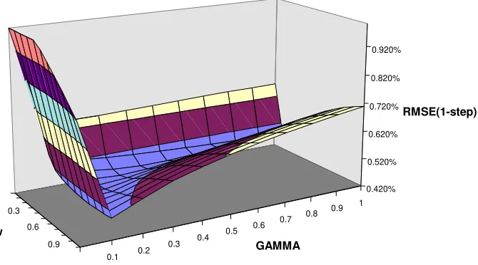
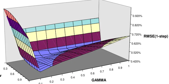
tightness and the tightness of the prior on cross lags was examined. Figures 1, 2 and 3
Table 4.1 BVAR Hyperparameters
Overall Tightness (γ) Relative Tightness(w)
SOE Model(BVAR1) 0.4 0.8
Augmented SOE(BVAR2) 0.3 0.3
in Appendix I, plot the 1-step ahead RMSE on all three models for values of γ and w
over the interval [ε, 1] where ε is an arbitrarily small number close to zero.23 From the
graph, it is relatively clear that too tight a prior leads to a dramatic reduction in the
forecasting performance of each model. For example, as γ tends toward zero, the
RMSE increases dramatically indicating that unless the random walk prior is revised in
the light of the significant historical interaction among the data forecasting
performance will not be optimal. Hence, an “extreme Bayesian” who is too certain of
his/her priors will forecast poorly. In the case of both the Augmented SOE (BVAR2)
and the Monetary Models (BVAR3), in Figures 2 and 3 respectively, there are clear
gains in terms of forecasting performance from being a “ moderate” Bayesian. Fixing
the cross lags parameter at a relatively high value of unity, it can be seen that there are
significant gains in terms of lowering the 1-step ahead forecast error from increasing
the overall tightness on the Minnesota prior. In the case of small open economy model
(BVAR1), the 1-step ahead forecasting performance is less sensitive to an increase in
the overall tightness given a relatively diffuse value for the tightness on cross lags.
This is far from surprising given that the Bayesian approach was conceived with a view
to solving the problem of over-parameterisation. Since the small open economy model
includes only three variables it is significantly less over-parameterised relative to the
other two models. In addition, placing too tight a restriction on cross lags reduces
forecasting performance of each model. As w tends toward zero, each model
approaches a set of univariate autoregressions. This also reduces inflation forecasting
accuracy thereby emphasising the gains from multivariate models which take account
of the interaction among the variables in each model in the production of “optimal”
inflation forecasts. In a similar manner to that described above, the sensitivity of
forecasting performance to changes in the hyperparameters at longer horizons was also
examined. The general conclusions which could be drawn from this, however, were
broadly consistent with the evidence for the one-step ahead errors depicted in Figures
1, 2 and 3. In general too tight a prior gives rise to a significant decline in forecast
performance at both long and short horizons. The final choice of hyperparameters,
which reflects the evidence reported above, is given in Table 4.1.
In order to compare the impact of the Bayesian approach to estimating the parameters
of each of the models, summary statistics are computed for the case where each VAR
is estimated using (i) unrestricted OLS where the variables are in log levels (LVAR1,
LVAR2 and LVAR3), (ii) unrestricted OLS where the variables are logged and then
differenced once (DVAR1, DVAR2, DVAR3) and (iii) the symmetric Minnesota prior that all variables are random walks with drift (BVAR1, BVAR2 and BVAR3). Also
reported for the purpose of comparison is the forecast performance of an AR(5) model
for the consumer price level. In addition, the forecasting performance for each model
under a general Minnesota prior was examined. This takes account of the likely exogeneity of foreign prices for a small economy such as Ireland’s by tightening the
prior of zero on the coefficients for the other variables (domestic prices/wages, the
exchange rate, domestic credit etc.) in the equation for foreign prices. Hence, under
this general prior, the foreign price equation is equivalent to a univariate regression of
foreign prices on its own lags. The general prior did not, however, improve forecasting
performance of any model examined and the results are not reported in order to
conserve space.
4.4 Results
The summary statistics for the three variable SOE vector autoregression as well as the
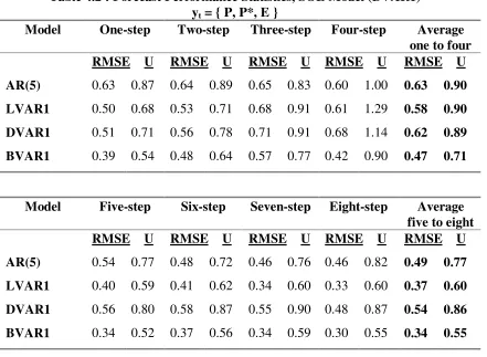
AR(5) model for the log of the HICP are given in Table 4.2. As indicated by the Theil
U statistics which are consistently less than unity, the AR(5) model outperforms the no
change or random walk model for the inflation rate. In addition, its relative
performance improves as the forecast horizon is extended. At relatively short-term
horizons, of up to four quarters out, the unrestricted VARs in levels or first differences
do not represent any significant improvement over the purely univariate time series
VAR in levels does significantly outperform either the VAR in differences or the
AR(5) model at longer horizons. The Bayesian VAR, however, outperforms all three
models discussed above. Over the short horizon, its average Theil statistic of 0.71 is
about 20% lower than that on any of the competing models. Given the RMSE of 0.39
per cent per quarter on its one step ahead forecast, the implied confidence intervals are
however still quite large. Under the assumption of normality, for example, the 68%
and 95% confidence interval would be approximately 0.80% and 1.60% per quarter.24
In addition, the unrestricted VAR in levels is not significantly worse than its Bayesian
counterpart on average at the longer horizon (5 to 8 quarters).25
24 The mean rate of inflation was 0.54% per quarter over the period 1992-1998.
25 Over the short horizon, BVAR1, does not perform as well as the ARIMA model for the HICP
Table 4.2 : Forecast Performance Statistics, SOE Model (BVAR1) yt = { P, P*, E }
Model One-step Two-step Three-step Four-step Average
one to four RMSE U RMSE U RMSE U RMSE U RMSE U
AR(5) 0.63 0.87 0.64 0.89 0.65 0.83 0.60 1.00 0.63 0.90
LVAR1 0.50 0.68 0.53 0.71 0.68 0.91 0.61 1.29 0.58 0.90
DVAR1 0.51 0.71 0.56 0.78 0.71 0.91 0.68 1.14 0.62 0.89
BVAR1 0.39 0.54 0.48 0.64 0.57 0.77 0.42 0.90 0.47 0.71
Model Five-step Six-step Seven-step Eight-step Average
five to eight RMSE U RMSE U RMSE U RMSE U RMSE U
AR(5) 0.54 0.77 0.48 0.72 0.46 0.76 0.46 0.82 0.49 0.77
LVAR1 0.40 0.59 0.41 0.62 0.34 0.60 0.33 0.60 0.37 0.60
DVAR1 0.56 0.80 0.58 0.87 0.55 0.90 0.48 0.87 0.54 0.86
BVAR1 0.34 0.52 0.37 0.56 0.34 0.59 0.30 0.55 0.34 0.55
Table 4.3: Forecast Performance Statistics, Augmented SOE Model (BVAR2) yt = { P, P*, E, W, RS }
Model One-step Two-step Three-step Four-step Average
one to four RMSE U RMSE U RMSE U RMSE U RMSE U
LVAR2 0.83 1.13 0.76 1.01 0.84 1.14 0.72 1.54 0.79 1.21
DVAR2 0.80 1.11 0.77 1.07 0.76 0.97 0.71 1.19 0.76 1.09
BVAR2 0.49 0.66 0.53 0.70 0.57 0.77 0.39 0.83 0.49 0.74
Model Five-step Six-step Seven-step Eight-step Average
five to eight RMSE U RMSE U RMSE U RMSE U RMSE U
LVAR2 0.55 0.82 0.63 0.95 0.58 1.02 0.49 0.89 0.56 0.92
DVAR2 0.62 0.89 0.59 0.89 0.53 0.87 0.33 0.59 0.52 0.81
Forecast performance summary statistics for the Augmented SOE model are
contained in Table 4.3. The statistics are again calculated for the unrestricted VAR in
levels, the unrestricted VAR in differences and also the VAR estimated conditional on
the Minnesota prior. At the short horizon, with average Theil statistics of 1.21 and
1.09, both unrestricted VARs were less accurate than a naive model which assumes no
change in the inflation rate! In addition, their average RMSEs over the short horizon
are substantially higher than the simple AR(5) model reported in Table 4.2. These
findings underline the extreme problem of overfitting and the resulting deficiency
-from a forecasting point of view - of non-Bayesian versions of this five variable model
system. At the longer horizon, these unrestricted VARs do, however, outperform the
naive model based on the average of the 5-to-8 step ahead errors. Once again,
however, the Bayesian version of the Augmented SOE VAR represents a considerable
improvement in terms of forecasting accuracy relative to its unrestricted counterparts
at both long and short horizons. The absolute forecasting accuracy of the BVAR2
model actually improves over the longer horizon. The Augmented model (BVAR2)
does not however outperform the Bayesian version of the simple SOE model (BVAR1
from Table 4.2). At both the long and short horizons the average RMSEs on the
augmented model are in fact marginally greater than the simple SOE model. While it is
not possible to distinguish between the Bayesian version of these two models, this
finding suggests that there was little incremental information in either wages or retail
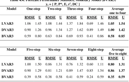
Finally, the summary statistics for the Monetary Model (BVAR3), which augments the
simple SOE BVAR1 to include both domestic credit and the short term nominal
interest rate, are reported in Table 4.4. Again, both unrestricted or non-Bayesian
versions of this VAR perform worse - at both long and short horizons - than a model
which predicts inflation on the basis of a “no change” assumption. Indeed, based on
the estimated RMSEs, the non-Bayesian estimates of the monetary model give rise to
the widest confidence intervals of all models which have been estimated thus far. The
68% confidence interval on the 1-step ahead forecast for the VAR in levels is, for
example, of the order of 2 per cent per quarter. Once again, however, the imposition
of Bayesian priors does result in a considerable improvement in forecast accuracy. At
both short and longer horizons, the RMSEs are approximately halved relative to the
unrestricted VARs in levels or first differences. The absolute accuracy of the Bayesian
VAR also improves as the horizon of the forecast is extended. At both the short and
the longer horizons, however, BVAR3 does not outperform the simple Bayesian model
which includes only domestic prices, the exchange rate and the import weighted
[image:30.595.85.522.80.359.2]measure of external prices (BVAR1).
Table 4.4: Forecast Performance Statistics, Monetary Model (BVAR3) yt = { P, P*, E, rs, DC }
Model One-step Two-step Three-step Four-step Average
one to four RMSE U RMSE U RMSE U RMSE U RMSE U
LVAR3 1.06 1.45 1.08 1.44 1.37 1.84 0.69 1.46 1.05 1.54
DVAR3 0.90 1.26 0.96 1.34 1.27 1.62 0.89 1.49 1.00 1.42
BVAR3 0.59 0.80 0.63 0.84 0.69 0.93 0.41 0.86 0.58 0.85
Model Five-step Six-step Seven-step Eight-step Average
five to eight RMSE U RMSE U RMSE U RMSE U RMSE U
LVAR3 1.00 1.50 0.86 1.31 0.76 1.32 0.60 1.11 0.80 1.31
DVAR3 0.90 1.29 0.81 1.21 0.89 1.47 0.85 1.54 0.86 1.37
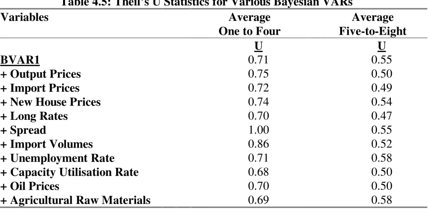
Finally, having compared and contrasted the three alternative vector autoregressive
models described above, the simple SOE model (BVAR1) is extended to include
various other indicators which were previously shown (in Table 4.1 ) to have some
degree of explanatory power. The results are reported in Table 4.5 in the form of the
average Theil Statistics from the one-to-four and five-to-eight forecast horizons.
Based on the average Theil statistics for the first four step ahead forecasts, none of
augmented models offer any significant improvement over the simple three variable
VAR (BVAR1). Indeed, in several cases the inclusion of an additional variable (such
as import volumes and the interest rate spread), gives rise to a substantial decrease in
the models performance over the short horizon.26 Over the longer horizon, based on
the average Theil from the five through eight step ahead forecasts, the inclusion of
import prices, new house prices, the long-term interest rate, the capacity utilisation
rate and oil prices give rise to some improvement in the models performance.
However, in light of the small sample from which the forecast error statistics are
calculated it would be unwise to consider these marginal differences as significant in
the statistical sense.
26 Henry and Peseran (1993) found a similar result for various VAR models of UK inflation. In
[image:31.595.90.522.465.676.2]particular, the addition of the unemployment rate or unit labour costs actually increased the RMSEs for inflation forecasts relative to a core model which included only three variables (inflation, changes in M0 and consumer confidence).
Table 4.5: Theil’s U Statistics for Various Bayesian VARs
Variables Average
One to Four
Average Five-to-Eight
U U
BVAR1 0.71 0.55
+ Output Prices 0.75 0.50
+ Import Prices 0.72 0.49
+ New House Prices 0.74 0.54
+ Long Rates 0.70 0.47
+ Spread 1.00 0.55
+ Import Volumes 0.86 0.52
+ Unemployment Rate 0.71 0.58
+ Capacity Utilisation Rate 0.68 0.50
+ Oil Prices 0.70 0.50
5. Conclusions
From the beginning of 1999, the Irish economy confronts a new environment in which
monetary policy will be set by the Governing Council of the European Central Bank.
In this new setting, forecasts of Irish inflation will continue to be required as an input
into monetary policy. In addition, in light of the macroeconomic constraints which
Economic and Monetary Union will impose, forecasts of inflation should arguably take
on an increased significance in the formulation of fiscal policy and also in the wage
-bargaining process. Unfortunately, most previous research on Irish inflation has
focused on testing particular economic theories and not on forecasting per se. It is therefore important that research efforts be directed toward the construction of
forecasting models which are optimal in the sense that they make use of all available
information and weight it according to its relevance in helping to predict future price
developments.
The objective of this paper was to focus on the performance of non-structural
dynamic multivariate time series models for forecasting Irish inflation. These models
are reduced form specifications which take account of important historical
relationships among a set of economic time series. However, in light of the large body
of evidence that the incorporation of prior beliefs can considerably improve forecasting
performance, the estimated models are also Bayesian in spirit. From a forecasting
point of view, the Bayesian approach can be viewed as a useful alternative to both
unrestricted VARs and also structural macroeconomic models. While Bayesian VARs
resemble unrestricted VARs in the form of the equations which are estimated, they
attempt to avoid the problem of overfitting by making use of prior beliefs which reduce
the data’s influence on the coefficient estimates. In addition, the extent of the data’s
influence on the estimated coefficients depends on the modeller’s level of confidence in
The evidence in the paper suggests that the imposition of Bayesian priors can
considerably improve the forecasting performance of the models which we have
examined. The paper examined three main vector autoregressive models for
forecasting Irish inflation. In each case, the Bayesian approach to parameter
estimation resulted in a dramatic improvement in forecasting performance relative to
unrestricted models. In one case (the monetary model), the confidence interval on the
one-step ahead forecast of inflation in an unrestricted VAR was almost three times as
large as that from its Bayesian counterpart. In general, however, forecasts of inflation
contain a high degree of uncertainty. Even the best performing Bayesian
autoregression had a 95% confidence interval of about 1.5 per cent per quarter based
on forecast errors computed over the period 1992-1998. The results are also
consistent with a number of previous studies in the Bank which stress a strong role for
the exchange rate and foreign prices as a determinant of Irish prices. Indeed, a simple
Bayesian VAR which included only these three variables (domestic prices, the nominal
exchange rate and external prices) proved to be quite robust relative to various
competing specifications augmented to include the impact of domestic demand, wages,
Appendix I
Figure 1
Sensitivity of Forecast Performance to Hyperparameters: BVAR1
0.3 0.6
0.9
0.1 0.2
0.3 0.4
0.5 0.6
0.7 0.8
0.9 1 0.375 0.475 0.575 0.675 0.775 0.875 0.975
RMSE(1-step)
w
GAMMA
Figure 2
Sensitivity of Forecast Performance to Hyperparameters: BVAR2
0.3 0.6
0.9
0.1 0.2
0.3 0.4
0.5 0.6
0.7 0.8 0.9 1
0.420% 0.520% 0.620% 0.720% 0.820% 0.920%
RMSE(1-step)
w
[image:34.595.121.456.470.656.2]Figure 3
Sensitivity of Forecast Performance to Hyperparameters: BVAR3
0.3 0.6
0.9
0.1 0.2
0.3 0.4
0.5 0.6
0.7 0.8
0.9 1 0.420% 0.520% 0.620% 0.720% 0.820% 0.920%
RMSE(1-step)
w
Appendix II
Description of Data and Sources
Domestic Price Series
Manufacturing output prices, export unit values, import unit values, average hourly earnings in the manufacturing sector were obtained from the Central Statistics Office database. Both new and second hand house prices were taken from various issues of the Housing Statistics Bulletin, compiled by the Department of the Environment.
Monetary/Financial Variables
The broad money stock (M3) and domestic credit series (DC) and the nominal
effective exchange rate (EER) were obtained from various issues of the Central Bank Quarterly Bulletin. Representative yields on short and long dated government stocks were used for short and long term interest rates. These were taken from the
International Financial Statistics (IFS) databank, lines 17860c and 17861 respectively.
Domestic Demand/Activity Variables
Retail Sales, industrial production, import volumes, exchequer tax revenues and the standardised unemployment rate were all obtained from CSO databank. The measure of capacity utilisation was taken from the IBEC/ESRI quarterly industrial survey.
External Prices
Both measures of external prices were obtained by weighting together the consumer price indices of the UK, the US, France, Germany, Italy, the Netherlands, Belgium, and Japan. The import weighted series was constructed using weights implied by the share of each of the above countries in total Irish imports. The trade weighted series was constructed using the average of import and export weights. All trade shares were obtained from the CSO Trade Statistics.
International Commodity Prices
References
Alberola E. and T. Tyrvainen (1998), “Is there scope for Inflation Differentials in EMU? An empirical Evaluation of the Balassa-Samuelson Model in EMU Countries”, Bank of Finland, Discussion Papers, 15/98.
Alvarez, L. J., F. C. Ballabriga and J. Jareno (1998), “A BVAR Model for the Spanish Economy”, Ch. 11 inMonetary Policy and Inflation in Spain, Malo de Mlina, Vinals and Gutierrez (eds), St. Martins Press, New York.
Artis, M. J. and W. Zhang (1990), “ BVAR Forecasts for the G-7”, International Journal of Forecasting, Vol. 6, pp. 349-362
Blejer, M. I and L. Leiderman (1981), “A monetary Approach to the crawling peg system: Theory and Evidence, Journal of Political Economy, Vol. 89, No. 1, pp. 289-296.
Callan, T. and J. Fitzgerald (1989), “Price Determination in Ireland: Effects of Changes in Exchange Rates and Exchange Rate Regimes”, The Economic and Social Review, Vol. 20, No. 2, January, pp. 165-188
Canova, F. (1995) ” Vector Autoregressive Models: Specification, Estimation, Inference and Forecasting”, Ch.2 in Handbook of Applied Econometrics , M. H. Peseran and M. Wickens (eds.), Oxford., pp. 73-138.
Cecchetti, S. (1995) “Inflation Indicators and Inflation Policy”, NBER Macroeconomics Annual 1995, The MIT Press, Cambridge MA, pp. 189-219.
Davidson, R. and J. G. McKinnon (1993), Estimation and Inference in Econometrics, Oxford University Press
Doan (1992) RATS User’s Manual Version 4.0, Estima.
Doan, T., R. Litterman and C. Sims (1984), “Forecasting and Conditional Projection Using Realistic Prior Distributions”, Econometric Reviews, Vol. 3, No. 1, pp. 1-100.
Dotsey, M and P. Ireland (1996), “The Welfare Cost of Inflation in General Equilibrium”, Journal of Monetary Economics, Vol. 37, pp. 29-47.
Dua, P. and S. C. Ray (1995) “ A BVAR model for the Connecticut Economy”, Journal of Forecasting, Vol. 14, Number 3, May, pp. 167-180.
Engle, R. F. and B. S. You (1987), “Forecasting and Testing Cointegrated Systems”, Journal of Econometrics, 35, pp. 143-59.
Feldstein, M. “The costs and benefits of going from low inflation to price stability”, NBER Working Paper No. 5469, February.
Hamilton, J. D. (1994) Time Series Analysis, Princeton University Press, Princeton, New Jersey.
Henry, S.G. B. and B. Peseran (1993), “ VAR Models of Inflation”, Bank of England Quarterly Bulletin, pp. 231-239.
Kenny, G. and D. McGettigan (1999), “ Modelling Traded, Non-Traded and Aggregate Inflation in a Small Open Economy: The Case of Ireland”, The Manchester School, 67, pp. 60-88.
Litterman, R.B. (1986) “Forecasting with Bayesian Vector Autoregressions - Five Years of Experience”, Journal of Business and Economic Statistics, January 1986, Vol. 4, No. 1, pp. 25-38.
Litterman, R. B. (1984) “Forecasting and Policy Analysis with Bayesian Vector Autoregressive Models”, Federal Reserve Bank of Minneapolis, Quarterly Review, Fall, pp. 30-41.
Lutkepohl, H.(1991) Introduction to Multiple Time Series Analysis, Springer-Verlag Berlin, Heidelberg.
McNees, S. K. (1986), “The accuracy of two forecasting techniques: some evidence and an
interpretation”, New England Economic Review, Federal Reserve Bank of Boston, March, pp. 20-31.
McGettigan, D. (1995), “The Term Structure of Interest Rates in Ireland: Description and Measurement”, Central Bank of Ireland Technical Paper 1/RT/95, April.
Meyler, A, G. Kenny and T. Quinn (1998) "Forecasting Irish Inflation using ARIMA models", Central Bank of Ireland Technical Paper 3/RT/98, December.
Newey, W. K. and K. D. West (1987), A Simple Positive, Semi-Definite, Heteroskedasticity and Autocorrelation Consistent Covariance Matrix” , Econometrica, Vol. 55, No. 3, May, pp. 703-708.
Stockton, D. J. and J. E. Glassman (1987) “An Evaluation of the Forecasting Performance of Alternative Models of Inflation””, The Review of Economics and Statistics, pp. 108-117.
Theil, H. (1963), “ On the use of incomplete prior information in regression analysis”, Journal of the American Statistical Association, Vol. 58, pp. 401-414.
Webb (1995) “Forecast of Inflation from VAR models”, Journal of Forecasting, Vol. 14, No. 3, May, pp. 268-285.