Scalable Semantic Web Data Management Using Vertical
Partitioning
Daniel J. Abadi
MIT[email protected]
Adam Marcus
MIT[email protected]
Samuel R. Madden
MIT[email protected]
Kate Hollenbach
MIT[email protected]
ABSTRACT
Efficient management of RDF data is an important factor in real-izing the Semantic Web vision. Performance and scalability issues are becoming increasingly pressing as Semantic Web technology is applied to real-world applications. In this paper, we examine the reasons why current data management solutions for RDF data scale poorly, and explore the fundamental scalability limitations of these approaches. We review the state of the art for improving perfor-mance for RDF databases and consider a recent suggestion, “prop-erty tables.” We then discuss practically and empirically why this solution has undesirable features. As an improvement, we propose an alternative solution: vertically partitioning the RDF data. We compare the performance of vertical partitioning with prior art on queries generated by a Web-based RDF browser over a large-scale (more than 50 million triples) catalog of library data. Our results show that a vertical partitioned schema achieves similar perfor-mance to the property table technique while being much simpler to design. Further, if a column-oriented DBMS (a database archi-tected specially for the vertically partitioned case) is used instead of a row-oriented DBMS, another order of magnitude performance improvement is observed, with query times dropping from minutes to several seconds.
1.
INTRODUCTION
The Semantic Web is an effort by the W3C [8] to enable in-tegration and sharing of data across different applications and or-ganizations. Though called the SemanticWeb, the W3C envisions something closer to a global database than to the existing World-Wide Web. In the W3C vision, users of the Semantic Web should be able to issue structured queries over all of the data on the Inter-net, and receive correct and well-formed answers to those queries from a variety of different data sources that may have information relevant to the query. Database researchers will immediately recog-nize that building the Semantic Web requires surmounting many of the semantic heterogeneity problems faced by the database commu-nity over the years. In fact – as in many database research efforts – the W3C has proposed schema matching, ontologies, and schema repositories for managing semantic heterogeneity.
Permission to copy without fee all or part of this material is granted provided that the copies are not made or distributed for direct commercial advantage, the VLDB copyright notice and the title of the publication and its date appear, and notice is given that copying is by permission of the Very Large Data Base Endowment. To copy otherwise, or to republish, to post on servers or to redistribute to lists, requires a fee and/or special permission from the publisher, ACM.
VLDB ‘07,September 23-28, 2007, Vienna, Austria.
Copyright 2007 VLDB Endowment, ACM 978-1-59593-649-3/07/09.
One area in which the Semantic Web community differs from the relational database community is in its choice of data model. The Semantic Web data model, called the “Resource Description Framework,” [9] or RDF, represents data as statements about re-sources using a graph connecting resource nodes and their property values with labeled arcs representing properties. Syntactically, this graph can be represented using XML syntax (RDF/XML). This is typically the format for RDF data exchange; however, structurally, the graph can be parsed into a series of triples, each representing a statement of the form<sub ject,property,ob ject>, which is the notation we follow in this paper. These triples can then be stored in a relational database with a three-column schema. For example, to represent the fact that Serge Abiteboul, Rick Hull, and Victor Vianu wrote a book called “Foundations of Databases” we would use seven triples1:
person1 isNamed ‘‘Serge Abiteboul’’ person2 isNamed ‘‘Rick Hull’’ person3 isNamed ‘‘Victor Vianu’’ book1 hasAuthor person1
book1 hasAuthor person2 book1 hasAuthor person3
book1 isTitled ‘‘Foundations of Databases’’
The commonly stated advantage of this approach is that it is very general (almost any type of data can be expressed in this format – it’s easy to shred both relational and XML databases into RDF triples) and it’s easy to build tools that manipulate RDF. These tools won’t be useful if different users describe objects differently, so the Semantic Web community has developed a set of standards for ex-pressing schemas (RDFS and OWL); these make it possible, for example, to say that every book should have an author, or that the property “isAuthor” is the same as the property “authored.”
This data representation, though flexible, has the potential for se-rious performance issues, since there is only one single RDF table, and almost all interesting queries involve many self-joins over this table. For example, to find all of the authors of books whose title contains the word “Transaction” it is necessary to perform the five-way self-join query shown in Figure 1.
This query is potentially very slow to execute, since as the num-ber of triples in the library collection scales, the RDF table may well exceed the size of memory, and each of these filters and joins will require a scan or index lookup. Real world queries involve many more joins, which complicates selectivity estimation and query op-timization, and limits the benefit of indices.
As a database researcher, it is tempting to dismiss RDF, as the 1In practice, RDF uses Universal Resource Identifiers (URIs), which look like URLs
and often include sequences of numbers to make them unique. We use more readable names in our examples in this paper.
SELECT p5.obj
FROM rdf AS p1, rdf AS p2, rdf AS p3, rdf AS p4, rdf AS p5
WHERE p1.prop = ’title’ AND p1.obj ˜= ’Transaction’ AND p1.subj = p2.subj AND p2.prop = ’type’ AND p2.obj = ’book’ AND p3.prop = ’type’ AND p3.obj = ’auth’ AND p4.prop = ’hasAuth’ AND p4.subj = p2.subj AND p4.obj = p3.subj AND p5.prop = ’isnamed’ AND p5.subj = p4.obj;
Figure 1: SQL over a triple-store for a query that finds all of the authors of books whose title contains the word “Transaction”.
data model seems to offer inherently limited performance for little – or no – improvement in expressiveness or utility. Regardless of one’s opinion of RDF, however, it appears to have a great deal of momentum in the web community, with several international con-ferences (ISWC, ESWC) each drawing more than 250 full paper submissions and several hundred attendees, as well as enthusiastic support from the W3C (and its founder, Tim Berners-Lee.) Further, an increasing amount of data is becoming available on the Web in RDF format, including the UniProt comprehensive catalog of pro-tein sequence, function, and annotation data (created by joining the information contained in Swiss-Prot, TrEMBL, and PIR) [6] and Princeton University’s WordNet (a lexical database for the English language) [7]. The online Semantic Web search engine Swoogle [5] reports that it indexes 2,171,408 Semantic Web documents at the time of the publication of this paper.
Hence, it is our goal in this paper to explore ways to improve RDF query performance, since it appears that it will be an impor-tant way for people to represent data on (or about) the web. We focus on using a relational query processor to execute RDF queries, as we (and several other research groups [22, 23, 27, 34]) feel that this is likely to be the best performing approach. The gist of our technique is based on a simple and familiar observation to propo-nents of relational technology: just as with relations, RDF does not have to be a proposal for physical storage – it is merely a logical data model. RDF databases are free to store RDF data as they see fit – including in ways that offer much better performance than ac-tually storing collections of triples in memory or on disk.
We look at two different physical organization techniques for RDF data. The first, called theproperty tabletechnique, denormal-izes RDF tables by physically storing them in a wider, flattened rep-resentation more similar to traditional relational schemas. One way to do this flattening, as suggested in [23] and [33], is to find sets of properties that tend to be defined together; i.e., clusters of subjects tend to have these properties defined. For example, “title,” “author,” and “isbn” might all be properties that tend to be defined for sub-jects that represent book entities. Thus a table containing subject as the key and “title,” “author,” and “isbn” as the other attributes might be created to store entities of type “book.” This flattened property table representation will require many fewer joins to access, since self-joins on the subject column can be eliminated. One can use standard query rewriting techniques to translate queries over the RDF triple-store to queries over the flattened representation.
There are several issues with this property table technique, in-cluding:
NULLs.Because not all properties will be defined for all subjects in the subject cluster, wide tables will have (possibly many) NULLs. For very wide tables with many sparse attributes, the space over-head of these NULLs can potentially dominate the space of the data itself.
Multi-valued Attributes.Multi-valued attributes (such as a book
with multiple titles in different languages) and many-to-many rela-tionships (such as the book authorship relationship where a book can have multiple authors and an author can write multiple books) are somewhat awkward to express in a flattened representation. Anec-dotally, many RDF datasets make heavy use of multi-valued at-tributes, so this may be of more concern here than in other database applications.
Proliferation of union clauses and joins. In the above example, queries are simple if they can be isolated to querying a single prop-erty table like the one described above. But if, for example, the query does not restrict on property value, or if the value of the property will be bound when the query is processed, all flattened tables will have to be queried and the results combined with either complex union clauses, or through joins.
To address these limitations, we propose a different physical or-ganization technique for RDF data. We create a two-column table for each unique property in the RDF dataset where the first column contains subjects that define the property and the second column contains the object values for those subjects. For the library exam-ple, tables would be created for the “title,” “author,” “isbn,” etc. properties, each table listing subject URIs with their corresponding value for that property. Multi-valued subjects are thus represented as multiple rows in the table with the same subject and different val-ues. Although many joins are still required to answer queries over multiple properties, each table is sorted by subject, so fast (linear) merge joins can be used. Further, only those properties that are ac-cessed by the query need to be read offdisk (or from memory), saving I/O time.
The above technique can be thought of as a fully vertically par-titioned database on property value. Although vertically partition-ing a database can be done in a normal DBMS, these databases are not optimized for these narrow schemas (for example, the tu-ple header dominates the size of the actual data resulting in table scans taking 4-5 times as long as they need to), and there has been a large amount of recent work on column-oriented databases [19, 20, 29, 31], which are DBMSs optimized for vertically partitioned schemas.
In this paper, we compare the performance of different RDF stor-age schemes on a real world RDF dataset. We use the Postgres open source DBMS to show that both the property table and the ver-tically partitioned approaches outperform the standard triple-store approach by more than a factor of 2 (average query times go from around 100 seconds to around 40 seconds) and have superior scal-ing properties. We then show that one can get another order of mag-nitude in performance improvement by using a column-oriented DBMS since they are designed to perform well on vertically par-titioned schemas (queries now run in an average of 3 seconds).
The main contributions of this paper are: an overview of the state of the art for storing RDF data in databases, a proposal to verti-cally partition RDF data as a simple way to improve RDF query performance relative to the state of the art, a description of how we extended a column-oriented database to implement the verti-cal partitioning approach, and a performance evaluation of these different proposals. Ultimately, the column-oriented DBMS is able to obtain near-interactive performance (on non-trivial queries) over real-world RDF datasets of many millions of records, something that (to the best of our knowledge) no other RDF store has been able to achieve.
The remainder of this paper is organized as follows. In Section 2 we discuss the state of the art of storing RDF data in relational databases, with an extended look at the property table approach. In Section 3, we discuss the vertically partitioned approach and explain how this approach can be implemented inside a
column-oriented DBMS. In Section 4 we look at an additional optimization to improve performance on RDF queries: materializing path expres-sions in advance. In Section 5, we summarize the library benchmark we use for evaluating the performance of an RDF database, and then compare the performance of the different RDF storage approaches in Section 6. Finally, we conclude in Section 7.
2.
CURRENT STATE OF THE ART
In this section, we discuss the state of the art of storing RDF data in relational databases, with an extended look at the property table approach.
2.1
RDF In RDBMSs
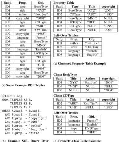
Although there have been non-relational DBMS proposals for storing RDF data [21], the majority of RDF data storage solutions use relational DBMSs, such as Jena [34], Oracle[23], Sesame [22], and 3store [27]. These solutions generally center around a giant triples table, containing one row for each statement. For example, the RDF triples table for a small library dataset is shown in Table 1(a).
Since URIs and literal values tend to be long strings (rather than those shown in the simplified example in 1(a)), many RDF stores choose not to store entire strings in the triples table; instead they store shortened versions or keys. Oracle and Sesame map string URIs to integer identifiers so the data is normalized into two tables, one triples table using identifiers for each value, and one mapping table that maps the identifiers to their corresponding strings. This can be thought of as dictionary encoding the string data. 3store does something similar, except the identifiers are created by applying a hash function to each string. Jena prefers to just dictionary encode the namespace prefixes in the URIs and only normalizes the partic-ularly long strings into a separate table.
Each of the above listed RDF storage solutions implements a multi-layered architecture, where RDF-specific functionality (for example, query translation) is performed in a layer above the RDBMS (which sits in the lowest layer). This removes any dependence on the particular RDBMS used (though Sesame will take advantage of specific features of an object relational DBMS such as Postgres to use subtables to model class and property subsumption relations). Queries are issued in an RDF-specific querying language (such as SPARQL [11] or RDQL [10]), converted to SQL in the higher level RDF layers, and then sent to the RDBMS which will optimize and execute the SQL query over the triple-store.
For example, the SPARQL query that attempts to get the title of the book(s) Joe Fox wrote in 2001:
SELECT ?title FROM table
WHERE { ?book author ‘‘Fox, Joe’’ ?book copyright ‘‘2001’’ ?book title ?title }
would get converted into the SQL query shown in Table 1(b) run over the data in Table 1(a).
Note that this simple query results in a three-way self-join over the triples table (in fact, another join will generally be needed if the strings are normalized into a separate table, as described above). If the predicates are selective, this 3-way join is not expensive (assum-ing the triples table is indexed – typically there will be indexes on all three columns). However, the less selective the predicates, the more problematic the joins become. As a result, both Jena and Ora-cle propose changes to the schema to reduce the number of joins of this type:property tables. We now examine these data structures in more detail.
Subj. Prop. Obj.
ID1 type BookType
ID1 title “XYZ”
ID1 author “Fox, Joe” ID1 copyright “2001”
ID2 type CDType
ID2 title “ABC”
ID2 artist “Orr, Tim” ID2 copyright “1985” ID2 language “French”
ID3 type BookType
ID3 title “MNO”
ID3 language “English”
ID4 type DVDType
ID4 title “DEF”
ID5 type CDType
ID5 title “GHI”
ID5 copyright “1995”
ID6 type BookType
ID6 copyright “2004”
(a) Some Example RDF Triples
SELECT C.obj. FROM TRIPLES AS A,
TRIPLES AS B, TRIPLES AS C WHERE A.subj. = B.subj.
AND B.subj. = C.subj. AND A.prop. = ‘copyright’ AND A.obj. = ‘‘2001’’ AND B.prop. = ‘author’ AND B.obj. = ‘‘Fox, Joe’’ AND C.prop. = ‘title’
(b) Example SQL Query Over RDF Triples Table From (a)
Property Table
Subj. Type Title copyright
ID1 BookType “XYZ” “2001”
ID2 CDType “ABC” “1985”
ID3 BookType “MNP” NULL
ID4 DVDType “DEF” NULL
ID5 CDType “GHI” “1995”
ID6 BookType NULL “2004”
Left-Over Triples
Subj. Prop. Obj.
ID1 author “Fox, Joe” ID2 artist “Orr, Tim” ID2 language “French” ID3 language “English”
(c) Clustered Property Table Example
Class: BookType
Subj. Title Author copyright
ID1 “XYZ” “Fox, Joe” “2001”
ID3 “MNP” NULL NULL
ID6 NULL NULL “2004”
Class: CDType
Subj. Title Artist copyright
ID2 “ABC” “Orr, Tim” “1985”
ID5 “GHI” NULL “1995”
Left-Over Triples
Subj. Prop. Obj.
ID2 language “French” ID3 language “English”
ID4 type DVDType
ID4 title “DEF”
(d) Property-Class Table Example
Table 1: Some sample RDF data and possible property tables.
2.2
Property Tables
Researchers developing the Jena Semantic Web toolkit, Jena2 [33, 34] proposed the use of property tables to speed up queries over triple-stores. They proposed two types of property tables. The first type, which we call aclustered property table, contains clusters of properties that tend to be defined together. For example, for the raw data in Table 1(a), type, title, and copyright date tend to be defined as properties for similar subjects. Thus, a property table containing these three properties as attributes along with subject as the table key can be created, which stores the triples from the original data whose property is one of these three attributes. The resulting prop-erty table, along with the left-over triples that are not stored in this property table, is shown in Table 1(c). Multiple property tables with different clusters of properties may be created; however, a key re-quirement for this type of property table is that a particular property may only appear in at most one property table.
The second type of property table, termed a property-class table, exploits the type property of subjects to cluster similar sets of sub-jects together in the same table. Unlike the first type of property table, a property may exist in multiple property-class tables. Table 1(d) shows two example property tables that may be created from the same set of input data as Table 1(c). Jena2 found property-class tables to be particularly useful for the storage of reified statements (statements about statements) where the class is rdf:Statement and the properties are rdf:Subject, rdf:Property, and rdf:Object.
Oracle [23] also adopts a property table-like data structure (they call it a “subject-property matrix”) to speed up queries over RDF triples. Their utilization of property tables is slightly different from Jena2 in that they are not used as a primary storage structure, but rather as an auxiliary data structure – a materialized view – that can
be used to speed up specific types of queries.
The most important advantage of the introduction of property tables to the triple-store is that they can reduce subject-subject self-joins of the triples table. For example, the simple query shown in Section 2.1 (“return the title of the book(s) Joe Fox wrote in 2001”) resulted in a three-way self-join. However, if title, author, and copy-right were all located inside the same property table, the query can be executed via a simple selection operator.
To the best of our knowledge, property tables have not been widely adopted except in specialized cases (like reified statements). One reason for this may be that they have a number of disadvan-tages. Most importantly, as Wilkinson points out in [33], while prop-erty tables are very good at speeding up queries that can be an-swered from a single property table, most queries require joins or unions to combine data from several tables. For example, for the data in Table 1, if a user wishes to find out if there are any items in the catalog copyrighted before 1990 in a language other than En-glish, the following SQL queries could be issued:
SELECT T.subject, T.object FROM TRIPLES AS T, PROPTABLE AS P WHERE T.subject == P.subject
AND P.copyright < 1990 AND T.property = ‘language’ AND T.object != ‘‘English’’
for the schema in 1(c), and
(SELECT T.subject, T.object FROM TRIPLES AS T, BOOKS AS B WHERE T.subject == B.subject
AND B.copyright < 1990 AND T.property = ‘language’ AND T.object != ‘‘English’’) UNION
(SELECT T.subject, T.object FROM TRIPLES AS T, CDS AS C WHERE T.subject == C.subject
AND C.copyright < 1990 AND T.property = ‘language’ AND T.object != ‘‘English’’)
for the schema in 1(d). As can be seen, join and union clauses get introduced into the queries, and query translation and plan gen-eration get complicated very quickly. Queries that do not select on class type are generally problematic for property-class tables, and queries that have unspecified property values (or for whom property value is bound at run-time) are generally problematic for clustered property tables.
Another disadvantage of property tables is that RDF data tends not to be very structured, and not every subject listed in the table will have all the properties defined. The less structured the data, the more NULL values will exist in the table. In fact, these representa-tions can be extremely sparse – containing hundreds of NULLs for each non-NULL value. These NULLs impose a substantial perfor-mance overhead, as has been noted in previous work [13, 16, 18].
The two problems with property tables are at odds with one an-other. If property tables are made narrow, with few property columns that are highly correlated in their value definition, the average value density of the table increases and the table is less sparse. Unfortu-nately, the likelihood of any particular query being able to be con-fined to a single property table is reduced. On the other hand, if many properties are included in a single property table, the num-ber of joins and union clauses per query decreases, but the numnum-ber of NULLs in the table increases (it becomes more sparse), bloating the table and wasting space. Thus there is a fundamental trade-off between query complexity as a result of proliferation of joins and
unions and table sparsity (and its resulting impact on query perfor-mance). Similar problems have been noted in attempts to shred and store XML data in relational databases [26, 30].
A third problem with property tables is the abundance of multi-valued attributes found in RDF data. Multi-multi-valued attributes are sur-prisingly prevalent in the Semantic Web; for example in the library catalog data we work with in Section 5, properties one might think of as single-valued such as title, publisher, and even entity type are multi-valued. In general, there always seem to be exceptions, and the RDF data model provides no disincentives for making proper-ties multi-valued. Further, our experience suggests that RDF data is often unclean, with overloaded subject URIs used to represent many different real-world entities.
Multi-valued properties are problematic for property tables for the same reason they are problematic for relational tables. They cannot be included with the other attributes in the same table un-less they are represented using list, set, or bag attributes. However, this requires an object-relational DBMS, results in variable width attributes, and complicates the expression of queries over these at-tributes.
In summary, while property tables can significantly improve per-formance by reducing the number of self-joins and typing attributes, they introduce complexity by requiring property clustering to be carefully done to create property tables that are not too wide, while still being wide enough to answer most queries directly. Ubiquitous multi-valued attributes cause further complexity.
3.
A SIMPLER ALTERNATIVE
We now look at an alternative to the property table solution to speed up queries over a triple-store. In Section 3.1 we discuss the vertically partitioned approach to storing RDF triples. We then look at how we extended a column-oriented DBMS to implement this approach in Section 3.2
3.1
Vertically Partitioned Approach
We propose storage of RDF data using a fully decomposed stor-age model (DSM) [24], a performance enhancing technique that has proven to be useful in a variety of applications including data ware-housing [13], biomedical data [25], and in the context of RDF/S, for taxonomic data [17, 32]. The triples table is rewritten intontwo column tables wherenis the number of unique properties in the data. In each of these tables, the first column contains the subjects that define that property and the second column contains the object values for those subjects. For example, the triples table from Table 1(a) would be stored as:
Type ID1 BookType ID2 CDType ID3 BookType ID4 DVDType ID5 CDType ID6 BookType Author
ID1 “Fox, Joe”
Title ID1 “XYZ” ID2 “ABC” ID3 “MNO” ID4 “DEF” ID5 “GHI” Artist
ID2 “Orr, Tim”
Copyright ID1 “2001” ID2 “1985” ID5 “1995” ID6 “2004” Language ID2 “French” ID3 “English”
Each table is sorted by subject, so that particular subjects can be located quickly, and that fast merge joins can be used to reconstruct information about multiple properties for subsets of subjects. The value column for each table can also be optionally indexed (or a second copy of the table can be created clustered on the value col-umn).
The advantages of this approach (relative to the property table approach) are:
not problematic in the decomposed storage model. If a subject has more than one object value for a particular property, then each dis-tinct value is listed in a successive row in the table for that property. For example, if ID1 had two authors in the example above, the table would look like:
Author
ID1 “Fox, Joe” ID1 “Green, John”
Support for heterogeneous records. Subjects that do not define a particular property are simply omitted from the table for that prop-erty. In the example above, author is only defined for one subject (ID1) so the table can be kept small (NULL data need not be explic-itly stored). The advantage becomes increasingly important when the data is not well-structured.
Only those properties accessed by a query need to be read. I/O costs can be substantially reduced.
No clustering algorithms are needed. This point is the basis be-hind our claim that the vertically partitioned approach is simpler than the property table approach. While property tables need to be carefully constructed so that they are not too wide, but yet wide enough to independently answer queries, the algorithm for creating tables in the vertically partitioned approach is straightforward and need not change over time.
Fewer unions and fast joins. Since all data for a particular prop-erty is located in the same table (unlike the propprop-erty-class schema of Figure 1(d)), union clauses in queries are less common. And al-though the vertically partitioned approach will require more joins relative to the property table approach, properties are joined using simple, fast (linear) merge joins.
Of course, there are several disadvantages to this approach. When a query accesses several properties, these two-column tables have to be merged. Although a merge join is not expensive, it is also not free. Also, inserts can be slower into vertically partitioned tables, since multiple tables need to be accessed for statements about the same subject. However, we have yet to come across an RDF appli-cation where the insert rate is so high that buffering the inserts and batch rewriting the tables is unacceptable.
In Section 6 we will compare the performance of the property table approach and the vertically partitioned approach to each other and to the triples table approach. Before we present these experi-ments, we describe how a column-oriented DBMS can be extended to implement the vertically partitioned approach.
3.2
Extending a Column-Oriented DBMS
The fundamental idea behind column-oriented databases is to store tables as collections of columns rather than as collections of rows. In standard row-oriented databases (e.g., Oracle, DB2, SQLServer, Postgres, etc.) entire tuples are stored consecutively (either on disk or in memory). The problem with this is that if only a few attributes are accessed per query, entire rows need to be read into memory from disk (or into cache from memory) before the pro-jection can occur, wasting bandwidth. By storing data in columns rather than rows (or inntwo-column tables for each attribute in the original table as in the vertically partitioned approach described above), projection occurs for free – only those columns relevant to a query need to be read. On the other hand, inserts might be slower in column-stores, especially if they are not done in batch.At first blush, it might seem strange to use a column-store to store a set of two-column tables since column-stores excel at storing big wide tables where only a few attributes are queried at once. However, column-stores are actually well-suited for schemas of this type, for the following reasons:
Tuple headers are stored separately. Databases generally store tuple metadata at the beginning of the tuple. For example, Postgres contains a 27 byte tuple header containing information such as in-sert transaction timestamp, number of attributes in tuple, and NULL flags. In contrast, the rest of the data in the two-column tables will generally not take up more than 8 bytes (especially when strings have been dictionary encoded). A column-store puts header infor-mation in separate columns and can selectively ignore it (a lot of this data is no longer relevant in the two column case; for exam-ple, the number of attributes is always two, and there are never any NULL values since subjects that do not define a particular property are omitted). Thus, the effective tuple width in a column-store is on the order of 8 bytes, compared with 35 bytes for a row-store like Postgres, which means that table scans perform 4-5 times quicker in the column-store.
Optimizations for fixed-length tuples. In a row-store, if any at-tribute is variable length, then the entire tuple is variable length. Since this is the common case, row-stores are designed for this case, where tuples are located through pointers in the page header (instead of address offset calculation) and are iterated through us-ing an extra function call to a tuple interface (instead of iterated through directly as an array). This has a significant performance overhead [19, 20]. In a column-store, fixed length attributes are stored as arrays. For the two-column tables in our RDF storage scheme, both attributes are fixed-length (assuming strings are dic-tionary encoded).
Column-oriented data compression. In a column-store, since each attribute is stored separately, each attribute can be compressed sep-arately using an algorithm best suited for that column. This can lead to significant performance improvement [14]. For example, the sub-ject ID column, a monotonically increasing array of integers, is very compressible.
Carefully optimized column merge code. Since merging columns is a very frequent operation in column-stores, the merging code is carefully optimized to achieve high performance [15]. For example, extensive prefetching is used when merging multiple columns, so that disk seeks between columns (as they are read in parallel) do not dominate query time. Merging tables sorted on the same attribute can use the same code.
Direct access to sorted files rather than indirection through a B tree. While not strictly a property of column-oriented stores, the in-creased dependence on merge joins necessitates that heap files are maintained in guaranteed sorted order, whereas the order of heap files in many row-stores, even on a clustered attribute, is only guar-anteed through an index. Thus, iterating through a sorted file must be done indirectly through the index, and extra seeks between index leaves may degrade performance.
In summary, a column-store vertically partitions attributes of a table. The vertically partitioned scheme described in Section 3.1 can be thought of as partitioning attributes from a wide universal table containing all possible attributes from the data domain. Con-sequently, it makes sense to use a DBMS that is optimized for this type of partitioning.
3.2.1
Implementation details
We extended an open source column-oriented database system (C-Store [31]) to experiment with the ideas presented in this pa-per. C-Store stores a table as a collection of columns, each col-umn stored in a separate file. Each file contains a list of 64K blocks with as many values as possible packed into each block. C-Store, as a bare-bones research prototype, did not have support for tem-porary tables, index-nested loops join, union, or operators on the string data type at the outset of this project, each of which had to
be added. We chose to dictionary encode strings similarly to Oracle and Sesame (as described in Section 2.1) where only fixed-width integer keys are stored in the data tables, and the keys are decoded at the end of each query using and index-nested loops join with a large strings dictionary table.
4.
MATERIALIZED PATH EXPRESSIONS
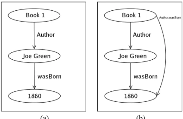
In all three RDF storage schemes described thus far (triples schema, property tables, and vertically partitioned tables), querying path ex-pressions (a common operation on RDF data) is expensive. In RDF data, object values can either be literals (e.g., “Fox, Joe”) or URIs (e.g.,http://preamble/FoxJoe). In the latter case, the value can be further described using additional triples (e.g.,<BookID1, Au-thor,http://preamble/FoxJoe>,<http://preamble/FoxJoe, wasBorn, “1860”>). If one wanted to find all books whose authors were born in 1860, this would require a path expression through the data. In a triples store, this query might look like:
SELECT B.subj
FROM triples AS A, triples AS B WHERE A.prop = wasBorn
AND A.obj = ‘‘1860’’ AND A.subj = B.obj AND B.prop = ‘‘Author’’
We need to perform a subject-object join to connect information about authors with information on the books they wrote.
In general, in a triples schema, a path expression requires (n−1) subject-object self-joins wherenis the length of the path. For a property table schema, (n−1) self-joins are also required if all prop-erties in the path expression are included in the table; otherwise the property table needs to be joined with other tables. For the verti-cally partitioned schema, the tables for the properties involved in the path expression need to be joined together; however these are joins of the second (unsorted) column of one table with the first column of the other table (and are hence not merge joins).
(a) (b)
Figure 2: Graphical presentation of subject-object join queries.
Graphically, the data is modeled as shown in Figure 2(a). Here we use the standard RDF semantic model where subjects and ob-jects are connected by labeled directed edges (properties). The path expression join can be observed through theauthorandwasBorn properties. If we could store the results of following the path ex-pression through a more direct path (shown in Figure 2(b)), the join could be eliminated:
SELECT A.subj FROM proptable AS A,
WHERE A.author:wasBorn = ‘‘1860’’
Using a vertically partitioned schema, this author:wasBorn path expression can be precalculated and the result stored in its own two column table (as if it were a regular property). By precalculating the path expression, we do not have to perform the join at query time. Note that if any of the properties along the path in the path expres-sion were multi-valued, the result would also be multi-valued. Thus, this materialized path expression technique is easier to implement in a vertically partitioned schema than in a property table.
Inference queries (e.g., if X is a part of Y and Y is a part of Z then X is a part of Z), a very common operation on Semantic Web data, are also usually performed using subject-object joins, and can be accelerated through this method.
There is, however, a cost in having a larger number of extra ma-terialized tables, since they need to be recalculated whenever new triples are added to the RDF store. Thus, for only or read-mostly RDF applications, many of these materialized path expres-sion tables can be created, but for insert heavy workloads, only very common path expressions should be materialized.
We realize that a materialization step is not an automatic im-provement that comes with the presented architectures. However, both property tables and vertically partitioned data lend themselves to allowing such calculations to be precomputed if they appear on a common path expression.
5.
BENCHMARK
In this section, we describe the RDF benchmark we have devel-oped for evaluating the performance of our three RDF databases. Our benchmark is based on publicly available library data and a collection of queries generated from a web-based user interface for browsing RDF content.
5.1
Barton Data
The dataset we work with is taken from the publicly available Barton Libraries dataset [1]. This data is provided by the Simile Project [4], which develops tools for library data management and interoperability. The data contains records acquired from an RDF-formatted dump of the MIT Libraries Barton catalog, converted from raw data stored in an old library format standard called MARC (Machine Readable Catalog). Because of the multiple sources the data was derived from and the diverse nature of the data that is cat-aloged, the structure of the data is quite irregular.
We converted the Barton data from RDF/XML syntax to triples using the Redland parser [3] and then eliminated duplicate triples. We then did some very minor cleaning of data, eliminating triples with particularly long literal values or with subject URIs that were obviously overloaded to correspond to several real-world entities (more than 99% of the data remained). This left a total of 50,255,599 triples in our dataset, with a total of 221 unique properties, of which the vast majority appear infrequently. Of these properties, 82 (37%) are multi-valued, meaning that they appear more than once for a given subject; however, these properties appear more often (77% of the triples have a multi-valued property). The dataset provides a good demonstration of the relatively unstructured nature of Seman-tic Web data.
5.2
Longwell Overview
Longwell [2] is a tool developed by the Simile Project, which provides a graphical user interface for generic RDF data exploration in a web browser. It begins by presenting the user with a list of the values thetypeproperty can take (such asTextorNotated Musicin the library dataset) and the number of times each type occurs in the data. The user can then click on the types of data to further explore. Longwell shows the list of currently filtered resources (RDF
sub-jects) in the main portion of the screen, and a list of filters in panels along the side. Each panel represents a property that is defined on the current filter, and contains popular object values for that prop-erty along with their corresponding frequencies. If the user selects an object value inside one of these property panels, this filters the working set of resources to those that have that property-object pair defined, updating the other panels with the new frequency counts for this narrower set of resources.
We will now describe a sample browsing session through the Longwell interface. The reader may wish to follow the described path by looking at a set of screenshots taken from the online Long-well Demo we include in our companion technical report [12]. The path starts when the user selectsTextfrom thetypeproperty box, which filters the data into a list of text entities. On the right side of the screen, we find that popular properties on these entities include “subject,” “creator,” “language,” and “publisher.” Within each prop-erty there is a list of the counts of the popular objects within this property. For example, we find out that the German object value ap-pears 122 times and the French object value apap-pears 131 times un-der the language property. By clicking on “fre” (French language), information about the 131 French texts in the database is presented, along with the revised set of popular properties and property values defined on these French texts.
Currently, Longwell only runs on a small fraction of the Barton data (9375 records), as its RDF triple-store cannot scale to support the full 50 million triple dataset (we show this scalability limitation in our experiments). Our experiments use Longwell-style queries to provide a realistic benchmark for testing the designs proposed. Our goal is to explore architectures and schemas which can provide interactive performance on the full dataset.
5.3
Longwell Queries
Our experiments feature seven queries that need to be executed on a typical Longwell path through the data. These queries are based on a typical browsing session, where the user selects a few specific entities to focus on and where the aggregate results sum-marizing the contents of the RDF store are updated.
The full queries are described at a high level here and are pro-vided in full in the appendix as SQL queries against a triple-store. We will discuss later how we rewrote the queries for each schema.
Query 1 (Q1).Calculate the opening panel displaying the counts of the different types of data in the RDF store. This requires a search for the objects and counts of those objects with propertyType. There are 30 such objects. For example:Type:Texthas a count of 1,542,280, andType:NotatedMusichas a count of 36,441.
Query 2 (Q2).The user selectsType:Textfrom the previous panel. Longwell must then display a list of other defined properties for re-sources ofType:Text. It must also calculate the frequency of these properties. For example, theLanguageproperty is defined 1,028,826 times for resources that are ofType:Text.
Query 3 (Q3).For each property defined on items ofType:Text, populate the property panel with the counts of popular object values for that property (where popular means that an object value appears more than once). For example, the propertyEditionhas 8 items with value “[1st ed. reprinted].”
Query 4 (Q4).This query recalculates all of the property-object counts from Q3 if the user clicks on the “French” value in the “Lan-guage” property panel. Essentially this is narrowing the working set of subjects to those whoseTypeisTextandLanguageisFrench. This query is thus similar to Q3, but has a much higher-selectivity.
Query 5 (Q5).Here we perform a type ofinference. If there are triples of the form (X Records Y) and (Y Type Z) then we can
in-ferthatX is of type Z. HereX Records Y means thatXrecords information aboutY(for example,Xmight be a web page with in-formation onY). For this query, we want to find the inferred type of all subjects that have thisRecordsproperty defined that also origi-nated in the US Library of Congress (i.e. contain triples of the form (X origin “DLC”)). The subject and inferred type is returned for all non-Textentities.
Query 6 (Q6).For this query, we combine the inference first step of Q5 with the property frequency calculation of Q2 to extract in-formation in aggregate about items that are either directly known to be ofType:Text(as in Q2) or inferred to be ofType:Textthrough the Q5Recordsinference.
Query 7 (Q7).Finally, we include a simple triple selection query with no aggregation or inference. The user tries to learn what a particular property (in this casePoint) actually means by selecting other properties that are defined along with a particular value of this property. The user wishes to retrieve subject,Encoding, andType of all resources with aPointvalue of “end.” The result set indicates that all such resources are of the typeDate. This explains why these resources can have “start” and “end” values: each of these resources represents a start or end date, depending on the value ofPoint.
We make the assumption that the Longwell administrator has se-lected a set of 28 interesting properties over which queries will be run (they are listed in our technical report [12]). There are 26,761,389 triples for these properties. For queries Q2, Q3, Q4, and Q6, only these 28 properties are considered for aggregation.
6.
EVALUATION
Now that we have described our benchmark dataset and the queries that we run over it, we compare their performance in three diff er-ent schemas – a triples schema, a property tables schema, and a vertically partitioned schema. We study the performance of each of these three schemas in a row-store (Postgres) and, for the verti-cally partitioned schema, also in a column-store (our extension of C-Store).
Our goal is to study the performance tradeoffs between these rep-resentations to understand when a vertically partitioned approach performs better (or worse) than the property tables solution. Ul-timately, the goal is to improve performance as much as possible over the triple-store schema, since this is the schema most RDF store systems use.
6.1
System
Our benchmarking system is a hyperthreaded 3.0 GHz Pentium IV, running RedHat Linux, with 2 Gbytes of memory, 1MB L2 cache, and a 3-disk, 750 Gbyte striped RAID array. The disk can read cold data at 150-180 MB/sec.
6.1.1
PostgreSQL Database
We chose Postgres as the row-store to experiment with because Beckmann et al. [18] experimentally showed that it was by far more efficient dealing with sparse data than commercial database prod-ucts. Postgres does not waste space storing NULL data: every tuple is preceded by a bit-string of cardinality equal to the number of at-tributes, with ’1’s at positions of the non-NULL values in the tuple. NULL data is thus not stored; this is unlike commercial products that waste space on NULL data. Beckmann et al. show that Post-gres queries over sparse data operate about eight times faster than commercial systems.
We ran Postgres withwork mem=51200, meaning that 50 Mbytes of memory are dedicated to each sorting and hashing operation. This may seem low, but thework memvalue is considered per oper-ation, many of which are highly parallelizable. For example, when
multiple aggregations are simultaneously being processed during the UNIONed GROUP BY queries for the property table imple-mentation, a higher value ofwork memwould cause the query ex-ecutor to use all available physical memory and thrash. We set effec-tive cache sizeto 183500 4KB pages. This value is a planner hint to predict how much memory is available in both the Postgres and operating system cache for overall caching. Setting it to a higher value does not change the plans for any of the queries run. We turnedfsyncoffto avoid syncing the write-ahead log to disk to make comparisons to C-Store fair, since it does not use logging [31]. All queries were run at a READ COMMITTED isolation level, which is the lowest level of isolation available in Postgres, again because C-Store was not using transactions.
6.2
Store Implementation Details
We now describe the details of our store implementations. Note that all implementations feature a dictionary encoding table that maps strings to integer identifiers (as was described in Section 2.1); these integers are used instead of strings to represent properties, subjects, and objects. The encoding table has a clustered B+tree index on the identifiers, and an unclustered B+tree index on the strings. We found that all experiments, including those on the triple-store, went an order of magnitude faster with dictionary encoding.
6.2.1
Triple Store
Of the popular full triple-store implementations, Sesame [22] seemed the most promising in terms of performance because it pro-vides a native store that utilizes B+tree indices on any combination of subjects, properties, and objects, but does not have the overhead of a full database (of course, scalability is still an issue as it must perform many self-joins like all triple-stores). We were unable to test all queries on Sesame, as the current version of its query lan-guage, SeRQL, does not support aggregates (which are slated to be included in version 2 of the Sesame project). Because of this limi-tation, we were only able to test Q5 and Q7 on Sesame, as they did not feature aggregation. The Sesame system implements dictionary encoding to remove strings from the triples table, and including the dictionary encoding table, the triples table, and the indices on the tables, the system took 6.4 GBytes on disk.
On Q5, Sesame took 1400.94 seconds. For Q7, Sesame com-pleted in 79.98 seconds. These results are the same order of mag-nitude, but 2-3X slower than the same queries we ran on a triple-store implemented directly in Postgres. We attribute this to the fact that we compressed namespace strings in Postgres more aggres-sively than Sesame does, and we can interact with the triple-store directly in SQL rather than indirectly through Sesame’s interfaces and SeRQL. We observed similar results when using Jena instead of Sesame.
Thus, in this paper, we report triple-store numbers using the di-rect Postgres representation, since this seems to be a more fair com-parison to the alternative techniques we explore (where we also di-rectly interact with the database) and allows us to report numbers for aggregation queries.
Our Postgres implementation of the triple-store contains three columns, one each for subject, property, and object. The table con-tains three B+tree indices: one clustered on (subject, property, ob-ject), two unclustered on (property, object, subject) and (object, subject, property). We experimentally determined these to be the best performing indices for our query workload. We also maintain the list of the 28 interesting properties described in Section 5.3 in a small separate table. The total storage needs for this implemen-tation is 8.3 GBytes (including indices and the dictionary encoding table).
6.2.2
Property Table Store
We implemented clustered property tables as described in Sec-tion 2.1. To measure their best-case performance, we created a prop-erty table for each query containing only the columns accessed by that query. Thus, the table for Q2, Q3, Q4 and Q6 contains the 28 interesting properties described in Section 5.3. The table for Q1 stores only subject andTypeproperty columns, allowing for repe-titions in the subject for multi-valued attributes. The table for Q5 contains columns for subject,Origin,Records, andType. The Q7 table contains subject,Encoding,Point, andTypecolumns. We will look at the performance consequences of property tables that are wider than needed to answer particular queries in Section 6.7.
For all but Q1, multi-valued attributes are stored in columns that are integer arrays (int[]in Postgres), while all other columns are integer types. For single-valued attributes that are used as selection predicates, we create unclustered B+tree indices. We attempted to use GiST [28] indexing for integer arrays in Postgres2, but us-ing this access path took more time than a sequential scan through the database, so multi-valued attributes used as selection predicates were not indexed. All tables had a clustered index on subject. While the smaller tables took less space, the property table with 28 proper-ties took 14 GBytes (including indices and the dictionary encoding table).
6.2.3
Vertically Partitioned Store in Postgres
The vertically partitioned store contains one table per property. Each table contains a subject and object column. There is a clus-tered B+tree index on subject, and an unclustered B+tree index on object. Multi-valued attributes are represented as described in Sec-tion 3.1 through multiple rows in the table with the same subject and different object value. This store took up 5.2 GBytes (including indices and the dictionary encoding table).
6.2.4
Column-Oriented Store
Properties are stored on disk in separate files, in blocks of 64 KB. Each property contains two columns like the vertically partitioned store above. Each property has a clustered B+tree on subject; and single-valued, low cardinality properties have a bit-map index on object. We used the C-Store default of 4MB column prefetching (this reduces seeks in merge joins). This store took up 2.7 GBytes (including indices and the dictionary encoding table).
6.3
Query Implementation Details
In this section, we discuss the implementation of all seven bench-mark queries in the four designs described above.
Q1.On a triple-store, Q1 does not require a join, and aggregation can occur directly on the object column after the property=Type se-lection is performed. The vertically partitioned table and the column-store aggregate the object values for theTypetable. Because the property table solution has the same schema as the vertically parti-tioned table for this query, the query plan is the same.
Q2.On a triple-store, this query requires a selection on property=Type and object=Text, followed by a self-join on subject to find what other properties are defined for these subjects. The final step is an aggregation over the properties of the newly joined triples table. In the property table solution, the selection predicateType=Textis applied, and then the counts of the non-NULL values for each of the 28 columns is written to a temporary table. The counts are then selected out of the temporary table and unioned together to pro-duce the correct results schema. The vertically partitioned store and column-store select the subjects for which theTypetable has ob-2http://www.sai.msu.su/megera/postgres/gist/intarray/README.intarray
ject valueText, and store these in a temporary table,t. They then union the results of joining each property’s table withtand count all elements of the resulting joins.
Q3.On a triple-store, Q3 requires the same selection and self-join on subject as Q2. However, the aggregation groups by both property and object value.
The property table store applies the selection predicateType=Text as in Q2, but is unable to perform the aggregation on all columns in a single scan of the property table. This is because grouping must be per property and then object for each column, and thus each column must group by the object values in that particular column (a single GROUP BY clause is not sufficient). The SQL standard describes GROUP BY GROUPING SETS to allow multiple GROUP BY ag-gregation groups to be performed in a single sequential scan of a table. Postgres does not implement this feature, and so our query plan requires a sequential scan of the table for each property aggre-gation (28 sequential scans), which should prove to be expensive. There is no way for us to accurately predict how the use of group-ing sets would improve performance, but it should greatly reduce the number of sequential scans.
The vertical store and the column store work like they did in Q2, but perform a GROUP BY on the object column of each prop-erty after merge joining with the subject temporary table. They then union together the aggregated results from each property.
Q4.On a triple-store, Q4 has a selection for property=Language and object=Frenchat the bottom of the query plan. This selection is joined with theType Textselection (again a self-join on subject), before a second self-join on subject is performed to find the other properties and objects defined for this refined subject list.
The property table store performs exactly as it did in Q3, but adds an extra selection predicate onLanguage=French.
The vertically partitioned and column stores work as they did in Q3, except that the temporary table of subjects is further nar-rowed down by a join with subjects whoseLanguagetable has ob-ject=French.
Q5.On a triple-store, this requires a selection on property=Origin and object=DLC, followed by a self-join on subject to extract the other properties of these subjects. For those subjects with theRecords property defined, we do a subject-object join to get the types of the subjects that were objects of theRecordsproperty.
For the property table approach, a selection predicate is applied onOrigin=DLC, and theRecordscolumn of the resulting tuples is projected and (self) joined with thesubjectcolumn of the original property table. Thetypevalues of the join results are extracted.
On the vertically partitioned and column stores, we perform the object=DLC selection on theOriginproperty, join these subjects with theRecordstable, and perform a subject-object join on the Recordsobjects with theTypesubjects to attain the inferred types.
Note that as described in Section 4, subject-object joins are slower than subject-subject joins because the object column is not sorted in any of the approaches. We discuss how the materialized path ex-pression optimization described in Section 4 affects the results of this query and Q6 in Section 6.6.
Q6.On a triple-store, the query first finds subjects that are directly ofType:Textthrough a simple selection predicate, and then finds subjects that are inferred to be ofType Textby performing a subject-object join through the records property as in Q5. Next, it finds the other properties defined on this working set of subjects through a self-join on subject. Finally, it performs a count aggregation on these defined properties.
The property table, vertical partitioning, and column-store ap-proaches first create temporary tables by the methods of Q2 and Q5, and perform aggregation in a similar fashion to Q2.
0 50 100 150 200 250
Query Time (seconds)
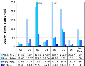
Triple Store 24.63 157 224.3 27.67 408.7 212.7 38.37 97 Prop. Table 12.66 18.37 579.8 28.54 47.85 101 6.1 38 Vert. Part. 12.66 41.7 71.3 35.49 52.34 84.6 13.25 36 C-Store 0.66 1.64 9.28 2.24 15.88 10.81 1.44 3 Q1 Q2 Q3 Q4 Q5 Q6 Q7 MeanGeo. 579.8 408.7
Figure 3: Performance comparison of the triple-store schema with the property table and vertically partitioned schemas (all three implemented in Postgres) and with the vertically parti-tioned schema implemented in C-Store. Property tables contain only the columns necessary to execute a particular query.
Q7.To implement Q7 on a triple-store, the selection on thePoint property is performed, and then two self-joins are performed to ex-tract theEncodingandTypevalues for the subjects that passed the predicate.
In the property table schema, the property table is narrowed down by a filter onPoint, which is accessed by an index. At this point, the other three columns (subject,Encoding,Type) are projected out of the table. BecauseTypeis multi-valued, we treat each of its two possible instances per subject separately, unioning the result of per-forming the projection out of the property table once for each of the two possible array values ofType.
In the vertically partitioned and column-store approaches, we join the filteredPointtable’s subject with those of theEncoding andTypetables, returning the result.
Since this query returns slightly less than 75,000 triples, we avoid the final join with the string dictionary table for this query since this would dominate query time and is the same for all four approaches. We are exploring intelligent caching techniques to reduce the cost of this final dictionary decoding step for high cardinality queries.
6.4
Results
The performance numbers for all seven queries on the four archi-tectures are shown in Figure 3. All times presented in this paper are the average of three runs of the queries. Between queries we copy a 2 GByte file to clear the operating system cache, and restart the database to clear any internal caches.
The property table and vertical partitioning approaches both per-form a factor of 2-3 faster than the triple-store approach (the geo-metric mean3of their query times was 38 and 36 seconds respec-tively compared with 97 seconds for the triple-store approach4. C-Store added another factor of 10 performance improvement with a geometric mean of 3 seconds (and so is a factor of 32 faster than the triple-store).
3We use geometric mean – thenth root of the product ofnnumbers – instead of the
arithmetic mean since it provides a more accurate reflection of the total speedup factor.
4If we hand-optimized the triple-store query plans rather than use the Postgres default,
we were able reduce the mean to 79s; this demonstrates the fact that by introducing a number of self-joins, queries over a triple-store schema are very hard to optimize.
To better understand the reasons for the differences in perfor-mance between approaches, we look at the perforperfor-mance differences for each query. For Q1, the property table and vertical partitioning numbers are identical because we use the idealized property table for each query, and since this query only accesses one property, the idealized property table is identical to the vertically partitioned table. The triple-store only performs a factor of two slower since it does not have to perform any joins for this query. Perhaps sur-prisingly, C-Store performs an order of magnitude better. To under-stand why, we broke the query down into pieces. First, we noted that the type property table in Postgres takes 472MB compared to just 100MB in C-Store. This is almost entirely due to the fact that the Postgres tuple header is 27 bytes compared with just 8 bytes of actual data per tuple and so the Postgres table scan needs to read 35 bytes per tuple (actually, more than this if one includes the pointer to the tuple in the page header) compared with just 8 for C-Store.
Another reason why C-Store performs better is that it uses an index nested loops join to join keys with the strings dictionary ta-ble while Postgres chooses to do a merge join. This final join takes 5 seconds longer in Postgres than it does in C-Store (this 5 sec-ond overhead is observable in the other queries as well). These two reasons account for the majority of the performance diff er-ence between the systems; however the other advantages of using a column-store described in Section 3.2 are also a factor.
Q2 shows why avoiding the expensive subject-subject joins of the triple-store is crucial, since the triple-store performs much more slowly than the other systems. The vertical partitioning approach is outperformed by the property table approach since it performs 28 merge joins that the property table approach does not need to do (again, the property table approach is helped by the fact that we use the optimal property table for each query).
As expected, the multiple sequential scans of the property table hurt it in Q3. Q4 is so highly selective that the query results for all but C-Store are quite similar. The results of the optimal property table in Q5-Q7 are on par with those of the vertically partitioned option, and show that subject-object joins hurt each of the stores significantly.
On the whole, vertically partitioning a database provides a signif-icant performance improvement over the triple-store schema, and performs similarly to property tables. Given that vertical partition-ing in a row-oriented database is competitive with the optimal sce-nario for a property table solution, we conclude that they are the preferable solution since they are simpler to implement. Further, if one uses a database designed for vertically partitioned data such as Store, additional performance improvement can be realized. C-Store achieved nearly-interactive time on our benchmark running on a single machine that is two years old.
We also note that multi-valued attributes play a role in reducing the performance of the property table approach. Because we im-plement multi-valued attributes in property tables as arrays, simple indexing can not be performed on these arrays, and the GiST [28] indexing of integer arrays performs worse than a sequential scan of the property table.
Finally, we remind the reader that the property tables for each query are idealized in that they only include the subset of columns that are required for the query. As we will show in Section 6.7, poor choice in columns for a property table will lead to less-than-optimal results, whereas the vertical partitioning solution represents the best- and worst-case scenarios for all queries.
6.4.1
Postgres as a Choice of RDBMS
There are several notes to consider that apply to our choice of Postgres as the RDBMS. First, for Q3 and Q4, performance for
0 50 100 150 200 250 0 5 10 15 20 25 30 35 40 45 50 55
Query time (seconds)
Number of Triples (millions) Triple Store
C-Store Vertical Partitioning
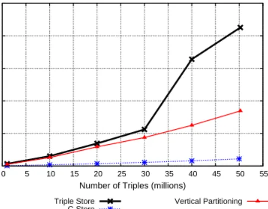
Figure 4: Query 6 performance as number of triples scale.
the property table approach would be improved if Postgres imple-mented GROUP BY GROUPING SETs.
Second, for the vertically partitioned schema, Postgres processes subject-subject joins non-optimally. For queries that feature the cre-ation of a temporary table containing subjects that are to be joined with the subjects of the other properties’ tables, we know that the temporary list of subjects will be in sorted order, as it comes from a table that is clustered on subject. Postgres does not carry this infor-mation into the temporary table, and will only perform a merge join for intermediate tuples that are guaranteed to be sorted. To simulate the fact that other databases would maintain the metadata about the sorted temporary subject list, we create a clustered index on the temporary table before the UNION-JOIN operation. We only in-cluded the time to create the temporary table and the UNION-JOIN operations in the total query time, as the clustering is a Postgres implementation artifact.
Further, Postgres does not assume that a table clustered on an attribute is in perfectly sorted order (due to possible modifications after the cluster operation), and thus can not perform the merge join directly; rather it does so in conjunction with an index scan, as the index is in sorted order. This process incurs extra seeks as the leaves of the B+tree are traversed, leading to a significant cost effect com-pared to the inexpensive merge join operations of C-Store.
With a different choice of RDBMS, performance results might differ, but we remain convinced that Postgres was a good choice of RDBMS, given that it handles NULL values so well, and thus enabled us to fairly benchmark the property table solutions.
6.5
Scalability
Although the magnitude of query performance is important, an arguably more important factor to consider is how performance scales with size of data. In order to determine this, we varied the number of triples we used from the library dataset from one mil-lion to fifty milmil-lion (we randomly chose what triples to use from a uniform distribution) and reran the benchmark queries. Figure 4 shows the results of this experiment for query 6. Both vertical par-titioning schemes (Postgres and C-Store) scale linearly, while the triple-store scales super-linearly. This is because all joins for this query are linear for the vertically partitioned schemes (either merge joins for the subject-subject joins, or index scan merge joins for the subject-object inference step); however the triple-store sorts the intermediate results after performing the three selections and be-fore performing the merge join. We observed similar results for all queries except queries 1, 4, and 7 (where the triple-store also scales linearly, but with a much higher slope relative to the vertically par-titioned schemes).