EOPTICS “Enhancement Ordering Points to Identify the Clustering Structure”

EOPTICS “Enhancement Ordering Points to

Identify the Clustering Structure”

Mahmoud E. Alzaalan

The Islamic University-Gaza Baghdad St, Alshijeya Gaza, Palestinian Territories

Raed T. Aldahdooh

The Islamic University-Gaza Salah-Eldeen St, Alzaytoon Gaza, Palestinian Territories

Wesam Ashour

The Islamic University-Gaza Khanyounis

Gaza, Palestinian Territories

ABSTRACT

Grouping a set of physical or abstract objects into classes of similar objects is a process of clustering. Clustering is very important technique in statistical data analysis. Among the clustering methods, density-based methods are critical because of their ability to recognize clusters with arbitrarily shape. In particular, OPTICS density-based method is an improvement upon DBSCAN. It addresses the major DBSCAN's weakness, which is the problem of detecting clusters in data of varying density. OPTICS defines the core distance which is the shortest distance from the core that contains the minimum number of points. Those points within the radius of the core distance may contain points far from the core than all the other points located within the same core distance. This algorithm computes the mean distance among the points within the core distance and the core itself and the resulting distance is considered as the new core distance.

General Terms

Data Clustering Algorithms, OPTICS, DBSCAN.

Keywords

Optimize OPTICS, Density-based clustering, core distance, mean distance.

1.

INTRODUCTION

Cluster analysis is the most popular tool in statistical data analysis which is widely applied in a variety of scientific areas such as data mining, pattern recognition, etc. Clustering is a very challenging task because of the lack of prior knowledge. Literature review reveals researchers‟ interest in the development of efficient clustering algorithms and their application in a variety of real-life situations. The main objective of clustering is grouping a set of physical or abstract objects into classes of similar objects. OPTICS [2] algorithm works in principle like extended DBSCAN algorithm for an infinite number of distance parameters ε‟ which are smaller than initial ε. It computes an augmented cluster-ordering of the database objects. The main advantage of OPTICS, when compared with DBSCAN clustering algorithm, is that OPTICS is not limited to one global parameter. Section 2 of this paper reviews various clustering algorithms and focuses on density-based algorithms. Section 3 reviews the basic concepts and steps of OPTICS algorithm. Section 4 describes our enhancement technique. Section 5 describes datasets and experiments with OPTICS, respectively.

2.

RELATED WORK

In the last decades many clustering algorithms were developed; these algorithms categorize into five main types [3]: Partitional, Hierarchical, Grid-based, Model-based and Density-based algorithms. In Partition-based algorithms,

cluster similarity is measured in regard to the mean value of the objects in a cluster, center of gravity, (K-Means [4]) or each cluster is represented by one of the cluster objects located near its center (K-Medoid [5]). Hierarchical algorithms such as BIRCH [6] and CURE [7] produce a set of nested clusters organized as a hierarchical tree. Grid-based algorithms such as STING [8], CLIQUE [9] and WaveCluster [10] are based on multi-level grid structure on which all clustering operations are performed. In Model-based algorithms (COB-WEB [11], etc.), a model is hypothesized for each of the clusters to find a model that best fits all other clusters.

The Density-based notion is a common approach for clustering which is based on the idea that objects which form a dense region should be grouped together into one cluster. Algorithms such as DBSCAN [12], OPTICS [2], DENCLUE [13] and CURD [14], core job of these algorithms is to find regions of high density in a feature space. To achieve better result of these algorithms, most of them need to have specific parameters or prior knowledge from users. Determining parameters is hard task, but have a significant influence on clustering results. Furthermore, for many real-data sets there is no global parameter setting that describes the intrinsic clustering structure accurately. DBSCAN was the first density-based method proposed for data clustering. This method comes with new definitions such as dense unit, neighborhood distance, and neighborhood radius. In this algorithm, to create a new cluster or extend an existing cluster, a neighborhood distance with radius ε must contain a minimum number of points denoted by “minimum points”. DBSCAN starts from a random point q and define neighborhood of q. If the neighborhood is contains a fewer number points than “minimum points”, then q is labeled as noise. Otherwise, a cluster is created of the resident points in q‟s neighborhood. Then the neighborhood of each neighbor is examined to see whether it can be added to the cluster. This process continues to extend an initial cluster as far as possible. If a cluster cannot be expanded further, DBSCAN chooses another unlabeled random point and repeats the process. This procedure is iterated until all points in the dataset have been clustered or labeled as noise.

Although DBSCAN shows very good results, it has some shortcomings. First, if the clusters have widely varying densities, DBSCAN is not able to handle them efficiently. Because all neighbors of a core object are checked, much time may be spent in dense clusters examining the neighborhoods of all points. If the data set contains clusters with various densities, DBSCAN selects ε large enough to cover the sparse areas, too. However, this selection is not optimal for dense regions.

for clustering data with variant density. ENDBSCAN and GMDBSCAN are variants of DBCSAN for identifying multi-density clusters, but their clustering results are highly sensitive to the parameter settings. LDBSCAN extends the local density factor to encode the local density information, which makes it capable of detecting multi-density clusters. However, it's not suitable for dataset with high diminution because of the difficulty of extend parameters. GDCIC is a grid-based density clustering algorithm, which is not able to handle high dimensional data sets because the size of grid is not easy to determine. NBC is an extension to DBSCAN based on a neighborhood-based density factor, which makes it capable of dealing with multi-density clusters. But its performance is highly sensitive to the density factor. To overcome DBSCAN weakness, OPTICS [2] has a noble idea of ordering points, also requires two inputs from the user just like DBSCAN. The two inputs are ε and the “minimum points”. OPTICS algorithm can‟t produce a clustering result explicitly but creates an augmented ordering of data set representing the density-based structures; from which embedded and multi-density clusters can be identified. This cluster-ordering contains information which is equivalent to the density-based clustering's corresponding to a broad range of parameter settings. It is a versatile basis for both automatic and interactive cluster analysis. OPTICS shows how automatically and efficiently extracts not only „traditional‟ clustering information, but also intrinsic clustering structure. For medium sized data sets, the cluster ordering can be represented graphically and for very large data sets, it introduces an appropriate visualization technique. Both are suitable for interactive exploration of the intrinsic clustering structure offering additional insights into the distribution and correlation of the data.

3.

BASIC CONCEPTS

3.1

OPTICS and Parameters Used In

Neighborhood Analysis

Let us consider that X={x1,x2,….,xn}, where xi , i=1,2,..,n. xi

is a vector of k features. Define Euclidian distance between any two points xi=[xi1,xi2,..,xik], xj =[xj1,xj2,..,xjk]  X is

which defined as:

𝑑 𝑥

, 𝑥

= 𝑥

− 𝑥

𝑘=1

1 2

Next paragraph, we will define some basic concepts used in OPTICS algorithm:

Definition-1 "Neighborhood": It is determined by computing Euclidian distance function or any other distance function between two points xi and xj, denoted by d(xi,xj).

Definition-2 "ε-Neighborhood set": The -neighborhood set of a point xi is defined by N (xi; ε) ={yX | d(xi, y) ≤ ε }.

Definition-3 "Core point": Let xi X is called a core point

with parameters ε if its neighborhood of a given ε has contained at least minimum number of point (fig.1).

Definition-3 "Directly density-reachable": Let xi, xj X.

xi is considered directly density-reachable from xj with respect

to the ε and minimum point if xj is a core point and xi is one of

the points contained in ε-neighborhood set points N(xi, ε) we

can note that all points in ε-neighborhood set can be directly density reachable from the core point only.

Definition-4 "Density-reachable": Let xi X, i = 1, ... , n. A

point xi is density reachable from a point xj with respect to ε

... , xn, xi = xj, xn = xi, such that xi+1 is directly

density-reachable from xi .

Definition-5 "Density-connected": Let xi, xj, xk X. A point

xi is density connected to a point xj with respect to ε and

minimum number of points if there is a core point xk such that

both xi and xj are density-reachable from xk with respect to ε

and minimum number of points.

Definition-6 "Border point": A point xi is a border point if it is not a core point but density-reachable from another core point.

Definition-7 "Density-based cluster": A cluster C is a non-empty subset of D satisfying the following „„Maximality‟‟ and „„Connectivity‟‟ requirements:

(1) Maximality: ∀ xi, xj : if xi ∈ C and xj is

density-reachable from xi with respect to ε and minimum

number of points, then xi ∈ C.

(2) Connectivity: ∀ xi, xj∈ C: xi is density-connected to xj

with respect to ε and minimum number of points. Definition-8 "Core-distance": Let xi ∈ Dataset X, MinPts is minimum number of point ∈ N, ε∈ R, and MinPts-distance (xi) be the distance from xi to its MinPts-nearest neighbor.

The core-distance of xi with respect to ε and MinPts is defined as follows:

UNDEFINED if Card (N(xi,ε)) <MinPts,

MinPts-distance(xi) Otherwise.

The core-distance of an point xi is simply the smallest distance ε‟ between xi and an object in its ε-neighborhood

such as xi would be a core object with respect to ε‟ if this

neighbor is contained in N (xi,ε).

Definition-9 "Reachability distance": Let xi ∈ Dataset X,

MinPts ∈ N and ε ∈ R. The reachability distance of xi with respect to ε and MinPts from an object xj∈ X is defined as

follows:

UNDEFINED if | N (xi,ε)| <MinPts,

Max (core-distance (xj), d(xi, xj)) Otherwise.

Intuitively, the reachability-distance of a point xi with respect to another point xj is the smallest distance such that xi is

directly density-reachable from xj if xj is a core point.

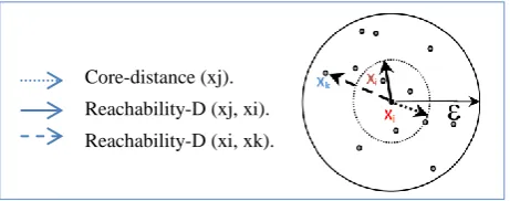
Considering a dataset X with ten points distributed in the clustering space; Figure 1 illustrates both concepts:

 The reachability distance of xi from xj equals the

core-distance of xj.

 Reachability distance of xk from xj equals the distance

between xk and xj.

Where xi, xj, and xk are points from dataset X, and input

parameters to the algorithm are ε and MinPts=5.

Figure 1: Two core-level and reachability-distance.

3.2

OPTICS Algorithm Steps

Step 2. Mark all the points in the dataset as unprocessed. Step 3. For each unprocessed point, find its neighbors w.r.t parameters ε and MinPts. Mark the point p as processed.

Core-distance (xj).

Reachability-D (xj, xi).

Step 6. If the core distance is undefined return to step 3, else go to step 7.

Step 7. Find the reachability distance for all neighbors and update the order seed depending on the new values.

Step 8.For all data in the order seed find the neighbor of the point.

Step 9. Mark the point as processed. Step 10. Set the core-distance for the point. Step 11. Add the point to the order file.

Step 12. If the core distance is undefined return to step 8, else go to step 13.

Step 13. Find the reachability distance for all neighbors and update the order seed depending on the new values.

End.

4.

PROPOSED METHOD

The main idea of OPTICS is using different values of epsilon to deal with different densities depending on concepts of reachability distance and core distance; the core distance was defined as the smallest distance ε‟ between a point and another point in its ε-neighborhood given that the first point is the core point with respect to ε‟. This means that within the radius ε‟ we must have an exact minimum number of points. Those points within the radius of the core distance may contain points far from the core than all the other points located within the same core distance. This algorithm computes the mean distance among the points within the core distance and the core itself and the resulting distance is considered as the new core distance.

Afterwards, the enhanced algorithm finds the reachability distance for all neighbor points within ε radius. For those points within ε‟ radius, the reachability distance equals the core distance, while for the rest points the reachability distance is the original distance.

Figure 2: illustrated enhancement in core-distance.

Figure 2 illustrates the concept of the enhanced algorithm. Assume that ε = 40 and the minimum number of points = 4, the outer circle is defined by the initial ε=40. For the square in the center if we search for ε‟ that is less than ε and contains 4 neighbors then we will have the dotted circle. The star is the point which satisfies the condition of core distance for the square point, but the density between the star and the other points within the dotted circle is different. Also, it may be outside those points‟ cluster. In the enhanced algorithm, the mean of the distances between the points within the dotted circle and the square point is calculated and the result is the new core distance.

5.

PERFORMANCE EVALUATION

5.1

Data Sets

With regard to the characteristics of data sets used in the evaluating the OPTICS performance algorithm after and before enhancements, the experiments depend on two different types of data sets (Artificial and Real datasets). Artificial datasets are used with two dimensions of features. Values of the generated artificial dataset are used to assess the level of the algorithm success. The real data sets used in the experiment are: IRIS and Mammographic Mass dataset. IRIS Data Set: This is perhaps the best known database to be found in the pattern recognition and clustering literature. Fisher's paper is a classic in the field and is referenced frequently to this day. The data set contains 3 classes of 50 instances each, where each class refers to a type of iris plant. One class is linearly separable from the other 2; the latter are not linearly separable from each other.

Mammographic Mass Data Set: The most effective method for breast cancer screening available today. This data set can be used to predict the severity (benign or malignant) of a mammographic mass lesion from BI-RADS attributes and the patient's age. It contains a BI-RADS assessment, the patient's age and three BI-RADS attributes together with the ground truth (the severity field) for 516 benign and 445 malignant masses that have been identified on full field digital mammograms collected at the Institute of Radiology of the University Erlangen-Nuremberg between 2003 and 2006.

5.2

Experiments Results

The experiment implementation is summarized in coding OPTICS and enhancing the concept of core-distance using Java programming language and thus, the algorithm runs on any platform. Moreover, the algorithm allows the user to load any cluster data sets from different file formats such as CSV, data or text files. There are several distance-measures can be used in OPTICS implementation such as the Euclidian, Manhattan or Cosine distance. For this version of OPTICS, Euclidian distance measures are used. OPTICS enhancement is compared with the original version of OPTICS in terms of clustering quality. A sensitivity analysis of OPTICS is provided with respect to the parameters ε and MinPts. Variant datasets were used to show the effects and performance development of the enhancement. For this purpose, 2 dimensional artificial datasets were applied, and then the enhanced algorithm was tested using real-world datasets.

5.2.1

Artificial Datasets

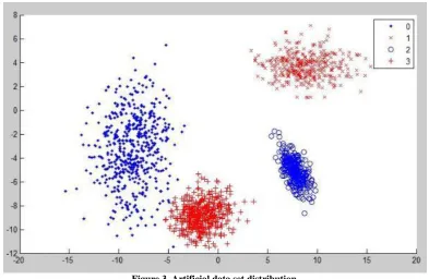
The dataset used contains 4 clusters as follows: cluster 0 from 1 to 528, cluster 1 from 529 to 876, cluster 2 from 877 to 1148 and cluster 3 from 1149 to 1572.

Figure 3 shows the distribution of values in the artificial dataset. Solid points denote cluster 0, crossed points denote cluster 1, circle points denote cluster 2 and plus points denote cluster 3.

Old core distance

Figure 3. Artificial data set distribution

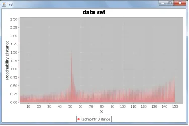
Figure 4 shows the visualization result of applying the enhanced algorithm, the value of epsilon=4 and minimum points = 6.

In this figure, the Y axis represents the reachability distance, while the X axis represents the resulting ordered points after applying the algorithm.

If this dataset was applied using the original OPTICS algorithm with ε=4 and minimum point = 6, the output would be three clusters while the enhanced algorithm output would be four clusters which is the right output.

Figure 4: reachability plot ε = 4, MinPoint=6.

5.2.2

Real Datasets

- Real Dataset 1. (IRIS):

A real dataset was used to measure the performance of the enhancement. Figure 5 shows the visualization result of applying the enhanced algorithm, the value of epsilon=5 and minimum points = 18.

- Real Datasets 2. (Mammographic Mass):

Figure 5: reachability plot ε = 5, MinPoint=18

Figure 6: reachability plot ε = 5, MinPoint=4

6.

CONCLUSION

Clustering is used in many fields such as data mining, knowledge discovery, statistics and machine learning. This paper presents enhancement to the concept of core-distance which is used in OPTICS clustering algorithm. The reason of this modification is to make OPTICS less sensitive to the variant density data. Experimental results demonstrate that the modification appears to give good performance when dealing with some datasets and gives the same performance of the original OPTICS algorithm with others datasets.

7.

REFERENCES

[1] J. Han, M. Kamber, 2001. Data Mining Concepts and Techniques, Morgan Kaufmann Publishers, San Francisco, CA, pp. 335–391.

[2] Ankerst M., Breunig M., Kriegel H.-P., Sander J, 99. OPTICS: Ordering Points To Identify the Clustering Structure.

[4] J. MacQueen, 1967. Some methods for classification and analysis of multivariate observations, in: Proceedings of the Fifth Berkeley Symposium on Mathematical Statistics and Probability, pp. 281–297.

[5] H. Vinod, 1969. Integer programming and the theory of grouping, Journal of the American Statistical Association vol. 64, pp. 506–519.

[6] T. Zhang, R. Ramakrishnan, M. Linvy, 1996. BIRCH: an efficient data clustering method for very large databases, in: Proceeding ACM SIGMOD International Conference on Management of Data, pp. 103–114.

[7] S. Guha, R. Rastogi, K. Shim, 1998. CURE: an efficient clustering algorithms for large databases, in: Proceeding ACM SIGMOD International Conference on Management of Data, Seattle, WA, pp. 73–84.

[8] W. Wang, J. Yang, R. Muntz, 1997. STING: a statistical information grid approach to spatial data mining, in: Proceedings of 23rd International Conference on Very Large Data Bases (VLDB), pp. 186–195.

[9] R. Agrawal, J. Gehrke, D. Gunopulos, and P. Raghavan,98. Automatic subspace clustering of high dimensional data for data mining applications.

[10]G. Sheikholeslami, S. Chatterjee, A. Zhang, 1998. WaveCluster: a multi-resolution clustering approach for very large spatial databases, in: Proceedings of International Conference on Very Large Databases (VLDB‟98), New York, USA, pp. 428–439.

[11]D. Fisher, 1987. Knowledge acquisition via incremental conceptual clustering, Machine Learning.

[12]Martin Ester, Hans-Peter Kriegel,1996. “A Density-based Algorithm for Discovering Clusters in Large Spatial Databases with Noise”.

[13]A. Hinneburg, D.A. Keim, 1998. An efficient approach to clustering in large multimedia databases with noise, in: Proceedings of 4th International Conference on Knowledge Discovery and Data Mining, New York City, NY, pp. 58–65.

[14]S. Ma, T.J. Wang, S.W. Tang, D.Q. Yang, J. Gao, A new fast clustering algorithm based on reference and density, in: Proceedings of WAIM, Lectures Notes in Computer Science, 2762, Springer, 2003, pp. 214–225.

[15]S. Roy, D.K, 2005.Bhattacharyya, an approach to find embe9ed clusters using density based techniques, in: Proceedings of the ICDCIT, Lecture Notes in Computer Science, vol. 3816, pp. 523–535.

[16]X. Chen, Y. Min, Y. Zhao, P. Wang, 2008.GMDBSCAN: multi-density DBSCAN cluster based on grid, in: IEEE International Conference on E-Business Engineering, pp. 780–783.

[17]L. Duan, L. Xu, F. Guo, J. Lee, B. Yan, 2007. A local-density based spatial clustering algorithm with noise, Information Systems 32

[18]S. Gao, Y. Xia, 2006. A grid-based density-confidence-interval clustering algorithm for multi-density dataset in large spatial database, in: International Conference on Intelligent Systems Design and Applications, vol. 1, pp. 713–717.

[19]S. Zhou, Y. Zhao, J. Guan, Z. Huang, 2005. A neighborhood-based clustering algorithm, in: Ninth Pacific-Asia Conference on Knowledge Discovery and Data Mining, Springer Press, Hanoi, , pp. 361–371.