Higher order volatility

Munich Personal RePEc Archive

Higher-order volatility

Carey, Alexander

1 December 2005

Online at

https://mpra.ub.uni-muenchen.de/4993/

HIGHER-ORDER VOLATILITY

Alexander Carey*

4 avenue de la Guillemotte 78112 Fourqueux, France [email protected]

December 1, 2005

* Alexander Carey is a graduate of Cass Business School, London. He has worked for Salomon Smith Barney New Zealand.

An often overlooked, but nonetheless important purpose of derivatives modelling is to provide practitioners with actionable measures of risk, the “thinkable quantities”

that Emanuel Derman has referred to.1 Dollar prices generally convey little information in the world of derivatives, and option pricing models are used — and abused — to convert them to and from a view on the market.

The historical risk measure, the Black and Scholes (1973) volatility, remains a favourite on trading floors in spite of well-known model-inconsistent biases, embodied in an implied volatility skew or smile. One popular approach to addressing these biases has

been to make volatility a function of time and the underlying asset price, as in the local volatility models of Dupire (1994), Derman and Kani (1994) and Rubinstein (1994). This offers a model-consistent fit to market prices, without introducing fundamentally new or

overly esoteric quantities into the risk interface, as can happen with other models.

In this paper, we present an alternative extension of volatility. Working first with a general stochastic process, we define a sequence of statistical parameters with an

1

intuitive gambling interpretation. We then derive moment formulae for the case when they are deterministic. Applied to a generic market quantity, the resulting risk interface features the familiar Black-Scholes handle on the variance of the underlying, along with “higher-order” analogues which capture departures from lognormality while retaining the look and feel of the original quantity. We provide snapshot implied values for the S&P 500 index options market.

1.

j

-TH ORDER VOLATILITY

We begin by considering a general adapted process (

X

_t) on a filtered probability space (

Ω

,

F F

,

( _t)

,

Q

). Let

δ

t

>

0

denote a finite period of time, and define

δ

δ

X

t

=

X

t+t

−

X

t, so that the relative change of the process over the interval t to

δ

+

t

t

reads

δ

X X

t t. We let

E

t

⋅

denote expectation conditional on

F

t, and

j

is a

generic positive integer.

Consider an agreement by which two parties undertake to exchange the amount

(

δ

X X

t t

)

j, as yet unknown but to be revealed imminently, and a predetermined amount

which we tentatively write in the form

(

Σ

,

)

×

δ

j

j t

t

. We suppose that both parties are in

possession of the information

F

_฀t, and that given this information, the agreement is a fair

gamble under the probability measure Q, by which we mean:

(

)

,

0

j _j

t t t j t

E

⎡

_⎢

δ

X X

− Σ

δ

t

⎤

_⎥

=

⎣

⎦

.

This leads us to formally define the quantity

Σ

j t, via the identity:

(

δ

)

δ

Σ

,

≡

j j

t t t

j t

E

X X

t

,

For an intuitive interpretation of this quantity, consider the following extrapolation. Assume for convenience that

m

×

δ

t

=

1

for some integer m, and consider a second agreement by which the original arrangement is extended to m

successive periods, but with the predetermined side remaining a fixed

Σ

j_{j t,}

δ

t

per period. In other words, the parties agree to exchange an unknown

(

δ

X

u

X

u

)

j and a

predetermined

Σ

j_{j t,}

δ

t

for each

u

=

t t

,

+

δ

t

,...,

t

+ −

1

δ

t

, with the unknown leg to be revealed imminently.2 Observing that the predetermined leg sums to

m

× Σ

j_{j t,}

δ

t

= Σ

j_{j t,} , suppose next that the process variable has changed exactly once between times t and

+

1

t

. Then if the relative change equals

Σ

j t, , the unknown leg equals the

predetermined leg and the parties are even. Thus, for such an agreement the quantity

Σ

j t, can be viewed as a break-even relative change. We shall refer to

Σ

j t, as

j

-th order

finite-period volatility.

Of particular interest will be the limit of vanishingly small

δ

t

, for which we define the quantity

σ

j t, via:

δ

σ

,

≡

lim

20

Σ

,

j j

t

j t j t,

again with

σ

j t, nonnegative when

j

is even. Equivalently,

σ

j t,

=

lim

δt20

Σ

j t, . We shall

refer to

σ

j t, as

j

-th order instantaneous volatility.

2. MOMENTS

Now in the general case the volatilities we have defined are stochastic. In the appendix we show that when the finite-period volatilities of orders one to n exist and are

2

deterministic, the

n

-th conditional moment of the process can be obtained as: τ

δ

+ =

⎡

_{⎛ ⎞⎟}

_⎜

⎤

⎢

_⎟

⎥

=

_⎢

+

_{⎜ ⎟}

_{⎜ ⎟}

Σ

_⎥

⎜⎝ ⎠

⎣

∑

⎦

∏

, 1

1

n j n n

t t t j u

u j

n

E X

X

t

j

, (1)

for any positive multiple

τ

of

δ

t

, where the product is over

u

=

t t

,

+

δ

t

,...,

t

+ −

τ

δ

t

. If we next suppose that there exists a

Δ >

0

such that this assumption holds for every

δ

t

≤ Δ

, then clearly the instantaneous volatilities, when they exist, are also

deterministic. Further, fixing

τ

>

0

and taking the limit

δ

t

2

0

in (1) yields:

τ

τ

σ

+ =

⎡

_{⎛ ⎞⎟}

_⎜

⎤

⎢

_⎟

⎥

=

_⎢

_{⎜ ⎟}

_{⎜ ⎟}

_⎥

⎜⎝ ⎠

⎣

∑

1

⎦

exp

n

j

n n

t t t j

j

n

E X

X

j

, (2)

where the

σ

_j, which are assumed to exist, are defined via:

,

1

t

j j

j j u

t

du

τ

σ

σ

τ

+

≡

∫

,

again with the convention that

σ

_j is nonnegative when

j

is even. We shall refer to

σ

_j as

j

-th order average volatility.3 _{We emphasise here that we have not established that}

deterministic instantaneous volatilities imply (2) in and of themselves. However, since the upper bound

Δ

in the above argument can be chosen arbitrarily small, this would seem to be more of a technical than a conceptual issue.

It is clear from (2) that the

n

-th moment of the process at time t is fully determined by the average volatilities of orders one to

n

. Thus, first-order volatility

σ

₁ determines the first moment, and we may take the view that given

σ

1, second-order

volatility

σ

2 governs the second moment, and so on. It is also apparent that if

σ

j

=

0

for every

j

>

2

, then

ln

(

X

t_+τ

X

t

)

is normally distributed (with mean

(

σ

1

−

12

σ τ

22

)

and variance

σ τ

22 ).4 Thus, nonzero values for higher-order average volatilities indicate

3

Admittedly a misnomer since it is the j-th power that is averaged. 4

and quantify deviations from the lognormal distribution. In particular,

σ

3 and

σ

4 govern

auxiliary skewness and kurtosis.

3. AN IMPLEMENTATION

We now take Q to be an equivalent martingale measure, (

F

_฀t) to be the market

information structure, and (

X

_t) to be an adapted market process. For expediency we limit ourselves to the basic equity setting, with

X

_t as the price at time t of a stock or index, with the money-market account as numeraire, and with the instantaneous dividend yield and riskless rate of interest both deterministic. In this context, it is easily verified that first-order volatility

σ

1,t equals the instantaneous cost of carry, which is

itself deterministic.

In what follows, we shall treat the volatilities exclusively as attributes of the market measure, to be implied from a set of option prices, rather than as inputs to a pricing scheme. We begin with the assumption that the volatilities of orders two through

n

are deterministic as per the previous section, and thus that the first

n

moments have

the form (2) (no assumption is necessary regarding higher orders). Note here that the first two model moments are now identical to those of the Black-Scholes model, with second-order volatility in the role of Black-Scholes volatility. We then propose to substitute a known distribution in place of the unknown one, fit it to the option prices, and compute the volatilities from the fitted statistics. For this it will prove convenient to use the canonical Merton (1976) jump-diffusion, which offers both a ready-to-use pricing capability and a reasonably good fit to market prices.

Poisson-driven jumps of size

κ

X

t at the rate

λ

. Here

σ

and

λ

are nonnegative

constants, and

ln 1

(

+

κ

) is normally distributed with mean

γ

−

1₂

δ

2 and variance

δ

2. Letting

m

_n and

m

n

′

denote the

n

-th moments (about zero) of

κ

and

1

+

κ

respectively, we have

m

1

=

e

γ

−

1

and

m

n

′ =

exp

[

n

γ

+

12

n n

(

−

1

)

δ

2

]

, and the

n

-th

conditional moment of the process reads:

( ) ( )

(

)

[

]

τ

λ

τ

σ τ

λτ

+

=

exp

−

1

+

12

−

1

2

+

′

−

1

n n

t t t n

E X

X

n b

m

n n

m

, (3)

where

b

is the instantaneous cost of carry. For convenience we recall the Merton (1973) version of the Black-Scholes formula for the price at time t of a plain vanilla option:

( ₁) ( ₂)

r b t

BSM

=

ε

e

− τ

_⎣

⎡

e X N

τ

ε

d

−

KN

ε

d

⎤

_⎦

,

with:

(

)

(

ν τ

)

ν τ

+

+

=

2 1 2 1

ln

X K

t

b

d

,

d

2

=

d

1

−

ν τ

,

where

K

is the exercise price, r is the rate of interest,

τ

is the time to expiration,

ν

is the volatility,

N

⋅

is the standard normal distribution function, and

ε

equals one for a call option, negative one for a put. The price of the same option under the jump-diffusion can then be written:

( ) 0

!

n n n

e

BSM

n

λτ

_λτ

∞ − =

∑

,

where

BSM

_n is the Black-Scholes-Merton formula, but with cost of carry

1 n

b

= −

b

λ

m

+

n

γ τ

and volatility

ν

_n

=

σ

2

+

n

δ τ

2 .5 _{As for the relationship between}

5

the jump-diffusion parameters and the volatilities, it is easily verified that (2) agrees with (3) when:

σ

jj

=

b

1

j=1

+

σ

2

1

j=2

+

λ

m

j

1

j≥2,

where

₁

_⋅ is the indicator function, and

m

j can be computed from the

m

k

′

via:

( ) −

=

⎛ ⎞⎟

⎜ ⎟

′

=

_{⎜ ⎟}

_{⎜ ⎟}

−

⎜⎝ ⎠

∑

0

1

j

j k

j k

k

j

m

m

k

.

4. AN EXAMPLE

For an example we turn to the S&P 500 (European-exercise) index options from the Chicago Board Options Exchange. The option price data is sourced from the exchange’s web-based quote service on May 13, 2005, time-stamped 14:43 ET (fifteen

minutes delayed), and consists of a snapshot of bid-ask quotes for all call and put contracts with under one year to expiration. The index level is 1,152.66. We discard all strikes for which the bid of either option is less than one-half a point, upon which for

each contract the bid and ask are averaged to produce a price estimate. Rates of interest are linearly interpolated from the most recent Libor curve. For each expiration, the estimation of the jump-diffusion parameters (cost of carry included) is carried out by

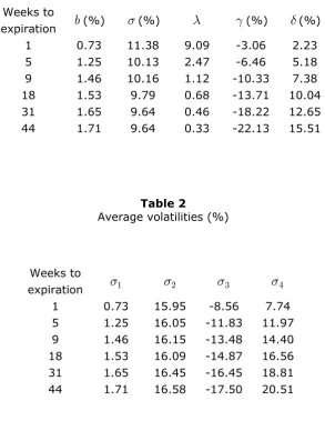
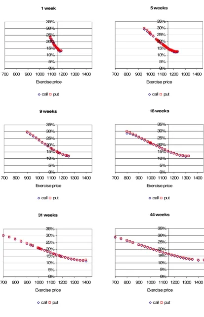
minimizing the sum of squared errors between market and model prices. Table 1 reports the estimated jump-diffusion parameters, and table 2 the corresponding average volatilities up to order four. Figure 1 shows the market price data in the form of implied

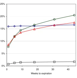
Black-Scholes volatilities (computed with the cost of carry from table 1), and figure 2 plots the implied average volatilities as per table 2.

Four aspects of these results stand out. The first is that the volatility estimates of

the cost of carry and to the Black-Scholes volatility.6 A second feature is that the two higher-order volatilities show themselves to be of the same order of magnitude as second-order volatility, making good on their initial promise. In absolute value, all three are within a two-percent range at the 18-week mark. A third feature is that third-order volatility is markedly negative, which is to be expected since equity indices tend to drop more sharply than they rise. Fourth and finally, the third and fourth-order volatility estimates show a marked expiration dependence, with sharply lower absolute values at the short end compared with the long one. On this feature we limit ourselves to two comments. First, our assumption that the volatilities are deterministic is clearly counterfactual, and should be expected to result in parameter bias. This is the unhappy lot of most financial models. However, as our second comment we ask whether it is reasonable to expect perfect rationality from derivatives markets. For example, the writing of short-dated, out-of-the-money vanilla options is an ordinarily profitable operation, which could lead some participants to take chances, wittingly or not, for comparatively less remuneration than is demanded at longer expirations. This kind of misjudgement is all the more plausible in the absence of suitable risk metrics beyond those measuring and pricing ordinary market variability.

5. CONCLUSION

We have introduced a set of risk measures which translate and convey the information in option market prices in a new way. Whether skew and smile exposures can be managed effectively via these quantities remains to be seen. The primary function that is envisaged for them is as an alternative to implied volatility surfaces for the

6

monitoring of market conditions. This risk interface is suitable for other products besides equity derivatives. It applies in a straightforward way to foreign exchange options, as well as interest-rate caplets and swaptions, subject to the standard parameterisations and assumptions.

APPENDIX

To establish (1), we note that:

(

+τ

)

(

δ

)

(

δ

)

=

⎡

_{⎛ ⎞⎟}

_⎜

⎤

⎢

_⎟

⎥

=

+

=

_⎢

+

_{⎜ ⎟}

_{⎜ ⎟}

_⎥

⎜⎝ ⎠

⎣

∑

⎦

∏

∏

1

1

1

n

n n j

t t u u u u

u u j

n

X

X

X

X

X

X

j

, (A1)

using the binomial theorem. Now

E

t

⋅ =

E E

t t_+δt

...

E

t_{+ −τ δ}t

⋅

, and assuming that the

Σ

, j j u

exist and are deterministic, taking expectations in (A1) and simplifying yields (1). To derive (2) we note that:

( )

δ

δ

δ

= =

⎡

⎤

⎛ ⎞

_⎟

⎛ ⎞

_⎟

⎜

_⎟

⎢

⎜

_⎟

⎥

+

_⎜

_⎜

_⎟

_⎟

Σ

=

_⎢

+

_⎜

_⎜

_⎟

_⎟

Σ

_⎥

⎜

⎜

⎝ ⎠

_⎣

⎝ ⎠

_⎦

∑

,

∑

, 1 1

1

exp

n n j j

j u j u

j j

n

n

t

o

t

t

j

j

,

where

o

( )

δ

t

represents terms which vanish with

δ

t

faster than

δ

t

(that is,

( )

δ

δ

→

0

o

t

t

as

δ

t

2

0

). Replacing in (1), we obtain:

(

+_τ

)

( )

δ

δ

=

⎡

_{⎛ ⎞⎟}

_⎜

⎤

⎢

_⎟

⎥

=

_⎢

+

_{⎜ ⎟}

_{⎜ ⎟}

Σ

_⎥

⎜⎝ ⎠

⎣

⎦

∑

∑

, 1

exp

n n _j

t t t j u

u j

n

E

X

X

o

t

t

j

. (A2)

Now by definition

Σ

j_{j u,}

→

σ

_{j u}j_, as

δ

t

2

0

, hence

∑

Σ

j_{j u,}

δ

→

σ τ

_jj

u

t

, and since

( )

δ

=

( )

δ τ δ

→

∑

0

u

REFERENCES

Bates, D. (1991) The crash of ’87: Was it expected? The evidence from options markets,

Journal of Finance46(3), 1009-1044.

Black, F. and M. Scholes (1973) The pricing of options and corporate liabilities, Journal of Political Economy 81(3), 637-654.

Derman, E. and I. Kani (1994) Riding on a smile, Risk 7(2), 32-39. Dupire, B. (1994) Pricing with a smile, Risk 7(1), 18-20.

Jarrow, R. and A. Rudd (1982) Approximate option valuation for arbitrary stochastic processes, Journal of Financial Economics10(3), 347-369.

Merton, R. (1973) Theory of rational option pricing, Bell Journal of Economics and Management Science 4(1), 141-183.

Merton, R. (1976) Option pricing when underlying stock returns are discontinuous,

Journal of Financial Economics3(1-2), 125-144.

Table 1

Jump-diffusion parameters

Weeks to

[image:13.595.150.444.143.541.2]

expiration

b

(%)

σ

(%)

λ

γ

(%)

δ

(%) 1 0.73 11.38 9.09 -3.06 2.23 5 1.25 10.13 2.47 -6.46 5.18 9 1.46 10.16 1.12 -10.33 7.38 18 1.53 9.79 0.68 -13.71 10.04 31 1.65 9.64 0.46 -18.22 12.65 44 1.71 9.64 0.33 -22.13 15.51

Table 2

Average volatilities (%)

Weeks to

expiration

σ

1

σ

2

σ

3

σ

4

[image:14.595.87.501.130.772.2]

Figure 1

S&P 500 implied Black-Scholes volatilities by expiration

1 week 0% 5% 10% 15% 20% 25% 30% 35%

700 800 900 1000 1100 1200 1300 1400

Exercise price call put 5 weeks 0% 5% 10% 15% 20% 25% 30% 35%

700 800 900 1000 1100 1200 1300 1400

Exercise price call put 9 weeks 0% 5% 10% 15% 20% 25% 30% 35%

700 800 900 1000 1100 1200 1300 1400

Exercise price call put 18 weeks 0% 5% 10% 15% 20% 25% 30% 35%

700 800 900 1000 1100 1200 1300 1400

Exercise price call put 31 weeks 0% 5% 10% 15% 20% 25% 30% 35%

700 800 900 1000 1100 1200 1300 1400

Exercise price call put 44 weeks 0% 5% 10% 15% 20% 25% 30% 35%

700 800 900 1000 1100 1200 1300 1400

Exercise price

[image:15.595.167.427.143.405.2]

Figure 2

Implied average volatilities

0% 5% 10% 15% 20% 25%

0 10 20 30 40

Weeks to expiration