Graph Neural Network for Minimum Dominating Set
GnanaJothi R.B.
Department of Mathematics V.V.Vanniaperumal College for Women, Virudhunagar-626 001
Tamil Nadu, India
Meena Rani S.M
Department of Mathematics V.V.Vanniaperumal College for Women, Virudhunagar-626 001
Tamil Nadu, India
ABSTRACT
The dominating set concept in graphs has been used in many applications. In large graphs finding the minimum dominating set is difficult. The minimum dominating set problem in graphs seek a set D of minimum number of vertices such that each vertex of the graph is either in D or adjacent to a vertex in D. In a graph on n nodes if there is a single node of degree n-1 then that single node forms a minimum dominating set. In the proposed work, a designed network called Graph Neural Network (GNN) is used to identify the node of degree N-1 in a graph having a single node of degree N-1 as it forms the minimum dominating set in the graph.. The network is simulated for graphs with nodes varying from 5 to 15. The state dimension of the input vectors are analyzed for better convergence. It has been found that the minimum dominating set was correctly identified from 80% to 90% of the graphs when the state dimension was 2 and 3. It has been observed that when the state dimension was 2, the convergence was fast as it requires minimum hidden neurons than other state dimensions. It has also been observed that when the state dimension was greater than 3, convergence requires hours of time and more number of hidden neurons. GNN was able to identify the minimum dominating set in a graph on n vertices which has a single node of degree n-1.
General Terms
Neural Networks
Keywords
Minimum dominating set, Graph neural network, State dimension, Feedforward neural network, Recursive neural network.
1.
INTRODUCTION
Graphs are used to represent many real life situations. The dominating set concept in graphs has been used in many applications. Positioning of Queens in a N-Queen problem, storing location information of the network nodes on mobile ad-hoc routing, are some of the applications of dominating set. In large graphs finding the minimum dominating set is difficult.
Graph Neural Networks have been recently proposed to process very general types of graphs, and can be considered an extension of Recursive Neural Networks[1]. In RNNs, the input graph to be directed and acyclic[2] [3] but GNNs have no limitations on types of graphs.
The GNN model implements a function
that maps a graph G and one of its nodes into an n-dimensional Euclidean space. The function depends on the node so that the classification depends on the properties of the node. Scarselli et al.[4] have used the GNN model to learn the rank of the web page. This approach simplifies the design of the page ranking algorithm by allowing automatic customization, based on training examples, of the rank to the particular needs of a search engine or internet user.GNNs have been proposed to process different types of graph theoretic problems such as subgraph matching [5], clique problem[6], Half Hot problem[6], Mutagenesis problem[5], and Tree depth problem[2]. Pucci et al. [7], have tested the GNN model on the Movie Lens data set, and pointed out some limitations of Graph Neural Networks when applied to recommender system. Muratore et al. [1] have applied GNN for sentence extraction in which the features of the sentences are taken as node labels and trained to produce the desired output on each node, so that GNN can automatically learn to predict the importance of each sentence. Uwents et al. [8] have compared and discussed GNN and Relational Neural Networks(RelNNs) on benchmarks that are commonly used by the relational learning community and have suggested that RelNNs and GNNs can be a viable approach for learning on relational data. Hongmei et al. [9] have proposed a neural network model to find the weakly connected dominating set in a wireless sensor network. Gabriele Monfardani et al. [10] have used GNN to locate face of a popular cartoon character in comics. Yong et al. [11] have proposed document mining using GNN. They have trained the network to encode and process a large set of XML formatted documents.
In this paper, we are using GNN model comprising of RNN(Transition Network) and FNN(output Network) to identify a minimum dominating set in an undirected graph with a single node of degree N-1. The structure of the paper is as follows. Section 2 describes minimum dominating set, Section 3 gives a brief description of GNN, Section 4 explains the generalized delta rule used in the weight updation procedure of the networks, Section 5 gives the training algorithm for generating the graphs and identifying the minimum dominating set in the training data. Experimental results are given in section 6.
2. MINIMUM DOMINATING SET
A dominating set D in a graph G=(V,E) is, a set D
V , such that every vertex v
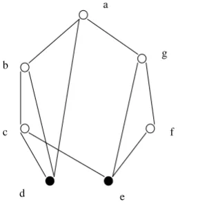
V \ D is adjacent to at least one vertex in D. In a graph, a dominating set with minimum cardinality is called the minimum dominating set. This is shown in figure 1. In a chess board, the positions of the minimum number of Queens that collectively dominate all 64 squares form a minimum dominating set in the corresponding graph. If a graph G with N nodes has a node v of degree N-1 then {v} is a minimum dominating set [12].3. GRAPH NEURAL NETWORKS
etc.). The state vector of a node with dimension s is computed using a feedforward neural network called Transition network which implements a local transition function fw.
n ne[n] ne[n]
w
n
f
l
,
x
,
l
x
(1)
] n [ n e
u w n u u
l
,
x
,
l
h
(2)For each node n, hw is a function of the state, label of the
neighboring node and its own label. Each node is associated with a feedforward neural network. Number of input patterns of the network depends on its neighbors. hw is considered to
be a linear function. When
n u u
n,u u n w l ,x ,l A x bh
where
b
n
R
sis defined as the output of feed forward neural network called bias network which implementss c w
:
R
R
,b
n
w
l
n , An,uRsxs is defined as the output of the feed forward neural network called forcing network which implements w:R2csRs2,))
l
,
x
,
l
(
(
resize
ne[n]
x
s
A
n,u
w n u uwhere
(
0
,
1
)
and resize operator allocates s2 elements in the output of forcing network to a s x s matrix.Let x, l denote the vector constructed by stacking all the states and all the node labels respectively of the graph. Then Equation (1) can be written as xFw
x,l . Banach fixedpoint theorem ensures the existence and the uniqueness of solution of Equation (1) in the iterative scheme for computing the state x(t1)Fw
x(t),l
where x(t) denotes the tthiteration of x. Thus the states are computed by iterating
n ne[n] ne[n]
w
n(t 1) f x (t),x ,l
x .
This computation is interpreted as a recurrent network that consists of units, transition networks, which compute fw the
units being connected as per graph topology.
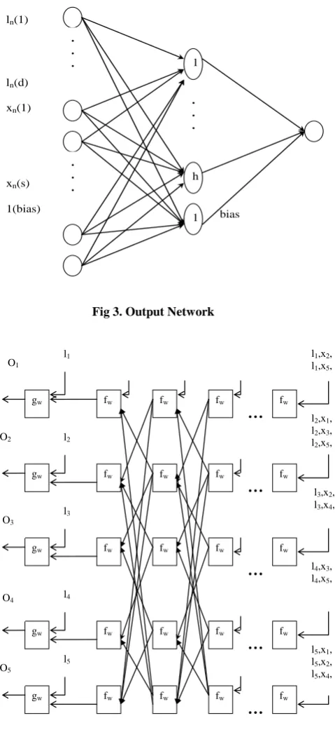
The output of each node of a graph is produced by a feed forward neural network called output network which takes as input the stabilized state of the node generated by the recurrent network and its label. For each node n, the output on is computed by the local output
function gw as
o
n
g
w
x
n
,
l
n
. Figure 3 and figure 4represent output network and GNN for the example graph figure 2.
[image:2.595.346.490.81.229.2]
Fig 1. Minimum Dominating Set
Fig 2. Example graph
4.GENERALIZED DELTA RULE
Weights of both transition network and output network are updated using Generalized Delta rule. In the standard Backpropagation algorithm, weights(w) are updated using gradient descent as
w e ) t (
w w
where
is the learningrate, ew the cost function given by mean square error
N
1 j
2 j j
w d y
xN 2
1
e where dj denotes the desired target
and yj the network output. Considering a fraction of the
previous weight change, the weight update rule can be taken
as
w
t 1w e t
w w
.
This weight updation rule is called the Generalized Delta rule. The fraction amount
considered in the rule is called momentum. This momentum term increases the rate of learning, maintaining stability.5. TRAINING ALGORITHM
Graphs with a single node of degree N-1 has to be generated as follows. Graphs with fixed number of nodes (N) has to be generated randomly. Each pair of nodes has to be connected with a certain probability. The resulting graph has to be checked to verify whether it is connected and if it is not, random edges are to be inserted until the condition is satisfied. The graph is then checked whether it has a single
l1
l2
l5
l4
l3
e b
c
d
node of degree N-1. If there is no such node, a random vertex is chosen and its degree is made N-1. If more than one vertex have degree N-1, a new graph has to be randomly generated to satisfy the condition.
Fig 3. Output Network
Fig 4. Graph Neural Network
1. Generate Graphs randomly with N nodes having a single node of degree N-1.
2. Label each node with dimension c by generating numbers randomly.
3. Assign a target 1 to the node of degree N-1, which constitutes the minimum dominating set and others 0.
4. Assume initial values of the state to be a zero s vector. 5. Generate bias network with c input neurons, h hidden neurons and s output neurons.
6. Generate single hidden layer transition network with 2*c+s input neurons h hidden neurons and s*s output neurons. 7. Generate output network with c+s+1 input neurons, h
hidden neurons and 1 output neuron.
8. Assign weights randomly for all the network from (0,1). 9. Calculate output of the bias network and Transition
network.
10. Stabilized states of the nodes are calculated by calling the Transition network recurrently.
11. Calculate the output of the output network by feeding the stabilized states and label of the node as input and then calculate mean square error.
12.Weights of all the networks are updated by backpropagation technique namely Generalized Delta rule.
13. Repeat steps 9 to 12 until desired accuracy is obtained.
6.RESULTS AND DISCUSSION
The GNN model was developed using Matlab code. Minimum dominating set for graphs on N nodes with a single node of degree N-1 was identified by this GNN model. Graphs were generated randomly with certain probability
. As we need only a single node of degree N-1, we set a large probability say
= 0.7. All the nodes were given integer labels in the range [0,10]. The data set consisted of 300 connected random graphs equally divided into a training set, a validation set and a test set. The results were averaged over 25 trails. Both the transition function hw and the output functiongw were implemented by three layered neural networks.
Number of hidden neurons of the networks vary depending on the number of nodes in the graph considered. Sigmoidal activation function was used in the hidden and output layers of the network. In this experiment, label dimension(c) was considered as 1. Termination condition was fixed as mean squared error 0.1. The weights of the networks were initialized randomly from (0, 1). Value of
used in the function of the transition network was randomly chosen between 0 and 1. When the value is more than 0.5, there was the possibility of dividing by zero in calculating the state vector xn . Hence
was set small as 0.005. The learningrate value used in the back propagation formula was 0.1. Momentum in these networks was considered as 0.1. The learning rate and parameter values were fixed by trial and error. The wrongly chosen values made the training diverge. The model was trained with various state dimensions starting from 2 to 9. The convergence was fast when the state dimension was 2. The model was tested for graphs with nodes 5 to 15. The number of hidden neurons was 5 for graphs with nodes 5 to 14 when the state dimension was 2 but it increased when the number of nodes of the graph was 15. When state dimension was 3, the number of hidden neurons was 5 for graphs with nodes 5 to 12 but when the number of nodes increased beyond 12, for fast convergence the number of hidden neurons were also increased. When the state dimension was greater than 3 it has been observed that the
1
h
1
. . .
. . .
. . .
ln(1)
ln(d)
xn(1)
xn(s)
1(bias) bias
fw
fw
fw
fw
fw
fw
fw
fw
l1,x2, l2
l1,x5, l5
fw
fw
fw
fw
fw
fw
fw
fw
gw
gw
gw
gw
l2,x1, l1
l2,x3, l3
l2,x5, l5
l1
l2
l3
l4
l3,x2, l2
l3,x4, l4
l4,x3, l3
l4,x5, l5
O1
O2
O3
O4
…
…
…
…
fw
fw
fw
fw
gw
…
O5
l5
l5,x1, l1
l5,x2, l2
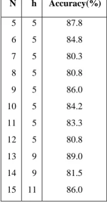
GNN consumed huge amount of time for convergence with more number of hidden neurons. Table 1 and 2 show the number of nodes in the graph, number of hidden neurons in the GNN and the accuracies obtained when state dimension was considered as 2 and 3 respectively. From the table it has been observed that the accuracy is more when s=2 and the number of hidden neurons needed for s=3 is more compared with s=2. When the termination condition
f used in stabilizing the state vector x is reduced, the number of epochs needed for the error to converge to 0.1 also decreased (See Table 3). The results where averaged over 10 trails.Table 1. Accuracies obtained when state dimension s=2
N h Accuracy(%)
5 6 7 8 9 10 11 12 13 14 15
5 5 5 5 5 5 5 5 5 5 9
88.6 86.8 81.8 82.8 90.4 88.6 84.1 81.2 89.5 82.7 87.0
Table 2. Accuracies obtained when state dimension s=3
N h Accuracy(%)
5 6 7 8 9 10 11 12 13 14 15
5 5 5 5 5 5 5 5 9 9 11
[image:4.595.118.216.238.437.2]87.8 84.8 80.3 80.8 86.0 84.2 83.3 80.8 89.0 81.5 86.0
Table 3. Number of epochs when termination condition is changed for the state vector
N f = 0.5 f = 0.1
5 6 7 8 9 10 11 12 13 14 15
17 20 35 40 42 48 50 62 110 123 199
6 5 7 9 9 19 29 13 19 22 12
7. CONCLUSION
In this paper, Minimum dominating set for the graph generated with N nodes and a single vertex of degree N-1 was identified using Graph neural network. GNN composed of Transition network, bias network and output network was trained to identify the minimum dominating set in the generated graph using GNN training algorithm and back propagation technique. Trained GNN was tested with newly generated graph. It has been found that, an average, the minimum dominating set was correctly identified from 80% to 90% of the graphs when the state dimension was 2 and 3. It has been observed that when s=2, the convergence was fast as it requires minimum hidden neurons than other state dimensions. Also it has been observed that when the state dimension was greater than 3, convergence requires hours of time and more number of hidden neurons. It has also been found that initial weights of the network, parameter in the transition network and learning parameter play an important role in convergence at training.
8.REFERENCES
[1] Muratore, D., Hagenbuchner, M., Scarselli, F., Tsoi, A.C., 2010. Sentence extraction by graph neural network, Proceedings of the 20th International conference on Artificial neural networks, Springer-Verlag, Berlin, Heidelberg, ISBN: 3-642-15824-2 978-3-642-15824-7 [2] Frasconi, M., Gori, M., Sperduti, A., 1998. A general
framework for adaptive processing of Data Structures. IEEE Trans. Neural Networks, 9: 768-786. DOI: 10.1109/72.712151
[3] Sperduti, A., Starita, A., 1997. Supervised Neural networks for the classification of structures. IEEE Trans. Neural Networks, 8: 714-735. DOI: 10.1109/72.572108. [4] Scarselli, F., Yong, S.L., Gori, M. Hagenbuchner, M.,
Tsoi, A.C., Maggini, M., 2005. Graph Neural Networks for Ranking Web Pages, in : Proceedings of the 2005 IEEE/WIC/ACM Int. Conf. on Web Intelligence.
[image:4.595.114.219.467.666.2][5] Scarselli, F., Gori, M., Tsoi, A.C., Hagenbuchner, M., Monfardini, G., 2009. The Graph neural network model. IEEE Trans. Neural Networks, 20: 61 - 78. DOI:10.1109/TNN.2008.2005605
[6] Scarselli, F., Gori, M., Tsoi, A.C., Hagenbuchner, M., Monfardini, G., 2009. Computational capabilities of Graph neural networks. IEEE Trans. Neural Networks, 20: 81 - 102.DOI:10.1109/TNN.2008.2005141
[7] Pucci, A., Gori, M., Hagenbuchner, M., Scarselli, F., Tsoi, A.C., 2006. Applications of Graph neural networks to large-scale recommender systems some results. Proceedings of International Multiconference on Computer Science and Information Technology pp: 189-195. www.proceedings2006.imcsit.org
[8] Uwents, W., Monfardini, G., Blockel, H., Gori, M., Scarselli, F., 2010. Neural networks for relational learning: an experimental comparison, Machine learning, DOI:10.1007/s10994-010-5196-5
[9] Hongmei, Zhenhuan Zhu, Erkki Makinen, 2009. A Neural network model to minimize the connected dominating set for self-configuration of wireless sensor networks. IEEE Trans. Neural Networks, 20: 973-982. DOI:10.1109/TNN.2009.2015088
[10] Manfordini G., Di Massa, V., Scarselli, F., Gori, M., 2006, Graph neural network for object localization, Fifth International workshop of the initiative for the evaluation of XML retrieval. DOI 10.1007/978-3-540-73888-6_43. [11] Yong, S.L., Hagenbuchner, M., Tsoi, A.C., Scarselli, F.,
Gori, M., 2007, Document mining using Graph neural network, Comparative evaluation of XML retrieval system, Lecture notes in Computer Science, 4518 : pp458 – 472.