Denoising of Poisson and Rician Noise from Medical Images using Variance Stabilization and Multiscale Transforms

Denoising of Poisson and Rician Noise from Medical

Images using Variance Stabilization and Multiscale

Transforms

V Naga Prudhvi Raj

T Venkateswarlu, PhD.

SV University, Tirupati, India.

ABSTRACT

Digital imaging in medicine is improving the medical standards since last few decades. The images acquired by various imag-ing modalities suffer from various kinds of noise in the acquisi-tion phase. The noise in the image decrease the contrast of the image and it becomes difficult to locate the tumours, lesions etc from these corrupted images. So the removal of noise from these images is very important. In this paper we developed the algo-rithms for the removal of Poisson noise in X-Ray Images and Rician noise in Magnetic Resonance Images. The noise in these modalities won’t follow the Gaussian distribution. The Poisson noise in X-ray images will follow the Poisson distribution and the noise in MR images is modeled as Rician noise. In this work we developed the algorithms using Discrete wavelet transform, Un-decimated wavelet transform, Dual tree Complex wavelet trans-form, Double Density discrete wavelet transform and Double den-sity dual tree complex wavelet transforms to decompose the im-age into multiple resolution levels along with the variance stabil-isation transforms to convert the Poisson noise and Rician noise into approximate gaussian noise. The performance of the algo-rithms were evaluated using PSNR (Peak signal to noise ratio), UQI (Universal quality index) and SSIM (Structural similarity in-dex) etc. The results show that the double density dual tree complex wavelet transform is performing well than the other transforms.

General Terms:

Multi Resolution Analysis, Wavelet Transforms, Variance Stabilization

Keywords:

Discrete Wavelet Transform, Dual tree complex wavelet trans-form, Double density wavelet transtrans-form, Wavelet shrinkage, Variance Stabilization.ifx

1. INTRODUCTION

Medical imaging became an integral part of medical diagnosis in present days. Various medical imaging modalities are developed for various applications since last few decades. These modalities are used to acquire the images of the anatomical structures within the body to be examined without opening the body. X-rays, Computed Tomography, Ultrasound, Magnetic resonance Imag-ing and Nuclear imagImag-ing are the popular modalities at present to diagnose the various diseases. However these modalities are suf-fering with a big problem called noise. Every modality is suffer-ing from noise in image acquisition and transmission stage such as Quantum noise in X-rays and Nuclear imaging, speckle noise in ultrasound imaging, Rician noise in Magnetic resonance imag-ing etc. The noise present in the images will degrade the contrast of the image and creates problems in the diagnostic phase. So

denoising is very important to remove the noise from these im-ages [16]. The noise may be additive or multiplicative depending on the modality used for medical image acquisition. The noise due to electronic components in the acquisition hardware will be modeled with Gaussian noise which is independent of data, the data dependent noise such as quantum noise in X-ray imag-ing is modeled with Poisson distribution, the speckle noise in ul-trasound imaging is modeled with Rayleigh distribution and the noise in MRI is modeled with Rician distribution. Here in this paper we are attempting to denoise the images corrupted with quantum noise in X-ray and Nuclear imaging and Rician noise in Magnetic Resonance Imaging [16, 12]. The mathematical mod-eling of degradation and restoration process is given as

g(x, y) =f(x, y)∗h(x, y) +η(x, y) (1) G(u, v) =F(u, v)H(u, v) +N(u, v) (2)

Where g(x,y) is the noisy and blurred observation, H is the blur-ring kernel and f(x,y) is the signal we are recoveblur-ring. In the case of denoising problem the blurring kernel will be dropped and the degradation model will be given as

g(x, y) =f(x, y) +η(x, y) (3) G(u, v) =F(u, v) +N(u, v) (4)

In the case of multiplicative noise the model is given as

g(x, y) =f(x, y)·η(x, y) (5)

2. MATHEMATICAL PROPERTIES OF NOISE 2.1 Poisson Noise

The noise in X-ray imaging and Nuclear Imaging (PET, SPECT) is modeled with Poisson noise. X-ray photons incident on a re-ceptor surface in a random pattern. We cannot force them to be evenly distributed over the receptor surface. One area of the re-ceptor surface may receive more photons than another area, even when both the areas are exposed to the same average x-ray in-tensity. In all medical imaging procedures using gamma or x-ray photons most of the image noise is produced by the random be-haviour of the photons that are distributed within the image. This is generally designated as quantum noise. Each individual pho-ton is a quantum (specific quantity) of energy. It is the quantum structure of an x-ray beam that creates quantum noise [10]. A Poisson model assume that each pixelxof an imagef(x)

is drawn from a Poisson distribution of parameterλ = f0(x) where is the original image to recover. The Poisson density is given as

P(f(x) =k) =λ k_e−λ

2.2 Rician Noise

Magnetic Resonance Imaging (MRI) is a non-invasive widely used modality in medical diagnosis such as cardiac related dis-eases and neurological disorders. The MRI imaging will suffer from low signal to noise ratio (SNR) or contrast to noise ratio (CNR) because of which the image analysis tasks such as seg-mentation, reconstruction and registration will become compli-cated. So the noise reduction in MR images is very important as a pre-processing task before going to image analysis and to improve the diagnostic quality of the images [10, 12].

Thermal noise is the major source of noise in MR imaging. The MR images are reconstructed from the raw data by applying the inverse Fourier transform to it. The signal component is present in both real and imaginary channels which are orthogonal to each other and are affected by additive white Gaussian noise. Hence the noise in the reconstructed date is complex white Gaussian noise. Normally the magnitude image of the reconstructed com-plex data is used for visual inspection. So the magnitude of the MR signal is the square root of the sum of the squares of the data present in real and imaginary channels, the noise is the square root of the two independent Gaussian variables. Hence the noise in MR images is no longer Gaussian.

LetAbe the pixel intensity in the absence of noise andMbe the observed or measured pixel intensity. In the presence of noise the probability distribution forMis given as

PM(M) = M σ2e

−(M2_+A2₎

2σ2 I0

A·M σ2

(7)

Whereσdenotes the standard deviation of the Gaussian noise in the real and imaginary images which is considered as equal here andIois the modified zeroth order of Bessel function of the

first kind. This is called as Rice density. For small values of SNR

(A/σ≤1)the rice distribution is far from being Gaussian and from ratios as small asA/σ = 3it starts to move towards the Gaussian distribution.

In the image regions where signal content is much less (approx-imately zero i.e.A = 0) only noise is present then the above equation is reduces to

PM(M) = M σ2e

−₍M2)

2σ2 (8)

This is well known as Rayleigh distribution. This distribution governs the noise in image regions where no NMR signal and only noise is present. The mean and variance of this distribution is given as

M =σ

r

π

2andσ

2

M =

2− π

2

σ2 ₍₉₎

These relations are useful in the estimation of the true noise power.

When the SNR is large then

PM(M)≈ 1 √

2πσ2e −1₍M−

√ A2 +σ2₎2

2σ2 (10)

From the above equations we can say that for image regions where large signal intensities are present the noise distribu-tion will be considered as a Gaussian distribudistribu-tion with mean

√

A2_+σ2_{and varianceσ}2

3. DENOISING USING MULTISCALE TRANSFORMS

In this section we want to use the multiscale transforms for the image denoising because they are very much useful to isolate the

discontinuites present in the image and to handle the nonstation-ary signals or time vnonstation-arying signals. The spatial domain filtering is succeeded to some extent by introducing the adaptivity in the filtering scheme through first order and higher order statistics at the cost of computational cost and leaving few artifacts such as ringings and smoothing the edges. In some filters the computa-tional cost is too high so that they are not optimal for real time filtering. To overcome these limitations lot of research was taken place in the last two decades.

The multiscale transforms such as gaussian and laplacian pyra-mids,steerable pyramids and wavelets are performing well in many image processing tasks by decomposing the images into multiple scales and using the benefit of sparsity and energy com-paction of the above transforms. In this paper we are denoising the images using wavelet transform, undecimated wavelet trans-form, dual tree complex wavelet transform and double density dual tree complex wavelet transform and compared the denoising performance with various quality metrics along with observing the effect of denoising on texture of the medical images which is a very important factor while choosing the denoising algorithm.

3.1 Discrete Wavelet Transform

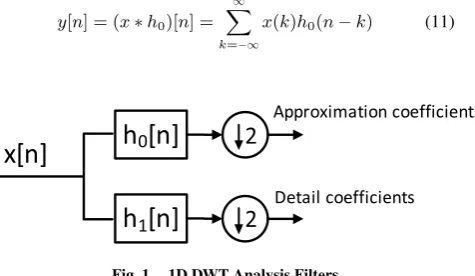
The DWT of a signalx(n)is calculated by passing it through a series of filters. First the samples are passed through a low pass filter with impulse responseh0(n)resulting in a convolution of the two [17]:

y[n] = (x∗h0)[n] = ∞

X

k=−∞

x(k)h0(n−k) (11)

Ś

΀Ŷ΁

Ϯ

Ś

΀Ŷ΁

Ϯ

dž΀Ŷ΁

ƉƉƌŽdžŝŵĂƚŝŽŶĐŽĞĨĨŝĐŝĞŶƚƐ

ĞƚĂŝůĐŽĞĨĨŝĐŝĞŶƚƐ

Fig. 1. 1D DWT Analysis Filters

The signal is also decomposed simultaneously using a high-pass filterh1(n). The outputs of the lowpass filter are approximation coefficients and highpass filter are detail coefficients. It is im-portant that the two filters are related to each other and they are known as a quadrature mirror filter. Since half the frequencies of the signal have now been removed, half the samples can be discarded according to Nyquist’s rule. The filter outputs are then subsampled by 2.

ylow[n] =

∞

X

k=−∞

x(k)h0(2n−k) (12)

yhigh[n] =

∞

X

k=−∞

x(k)h1(2n+ 1−k) (13)

2D DWT of the images can be implemented by applying 1D DWT along the rows of an image first and then applying 1D DWT on the columns of an image. When a wavelet transform is applied to an image the image is decomposed into four sub-bands as shown in the following figure. The LL band contains the approximation coefficients, LH band contains horizontal de-tails, HL band contains vertical details and HH band will contain the diagonal details [17].

dž΀Ŷ΁

ŚϬ΀Ŷ΁ Ϯ

Śϭ΀Ŷ΁ Ϯ

ŚϬ΀Ŷ΁ Ϯ

Śϭ΀Ŷ΁ Ϯ

ŚϬ΀Ŷ΁ Ϯ

Śϭ΀Ŷ΁ Ϯ

>,

,ŽƌŝnjŽŶƚĂůĞƚĂŝůŽĞĨĨŝĐŝĞŶƚƐ

,, ŝĂŐŽŶĂůĞƚĂŝůŽĞĨĨŝĐŝĞŶƚƐ

,> sĞƌƚŝĐĂůĞƚĂŝůŽĞĨĨŝĐŝĞŶƚƐ

>> ƉƉƌŽdžŝŵĂƚŝŽŶŽĞĨĨŝĐŝĞŶƚƐ

Fig. 2. Wavelet filtering of an Image

Directionality [20].To overcome these shortcomings a lot of re-search is on-going in present days. The Undecimated wavelet transform (UDWT) is the one of the solution by introducing the redundancy in the transform through the removal of decimation stage. The UDWT is shift invariant but it will increase the num-ber of coefficients so the computational complexity is high.

3.2 Dual tree complex wavelet Transform

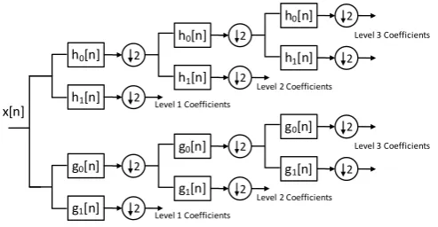
The dual-tree complex DWT of a signalx(n)is computed us-ing two critically-sampled DWTs in parallel on the same data as shown in the following figure. If the same filters used in the upper tree and lower tree nothing is gained. So the filters in this structure will designed in a specific way that the subbands of up-per DWT is interpreted as real part of complex wavelet transform and the lower tree as imaginary part. The transform is expansive by a factor 2 and shift invariant [20, 21].

dž΀Ŷ΁

ŚϬ΀Ŷ΁ Ϯ

Śϭ΀Ŷ΁ Ϯ

ŚϬ΀Ŷ΁ Ϯ

Śϭ΀Ŷ΁ Ϯ

ŚϬ΀Ŷ΁ Ϯ

Śϭ΀Ŷ΁ Ϯ

>ĞǀĞůϭŽĞĨĨŝĐŝĞŶƚƐ

>ĞǀĞůϮŽĞĨĨŝĐŝĞŶƚƐ

>ĞǀĞůϯŽĞĨĨŝĐŝĞŶƚƐ

ŐϬ΀Ŷ΁ Ϯ

Őϭ΀Ŷ΁ Ϯ

ŐϬ΀Ŷ΁ Ϯ

Őϭ΀Ŷ΁ Ϯ

ŐϬ΀Ŷ΁ Ϯ

Őϭ΀Ŷ΁ Ϯ

>ĞǀĞůϭŽĞĨĨŝĐŝĞŶƚƐ

>ĞǀĞůϮŽĞĨĨŝĐŝĞŶƚƐ

>ĞǀĞůϯŽĞĨĨŝĐŝĞŶƚƐ

Fig. 3. Dualtree DWT 1D Analysis Filters

The dual tree complex wavelet transform is implemented by de-signing the filter banks such a way that the filters in the second tree are the Hilbert transform of the first tree filters. That is in dual tree complex wavelet transform the filter sets in the first tree and second tree are forming a Hilbert transform pair. Let the filtersh0(n), h1(n)represents the CQF (conjugate quadrature filter) pair. That is

X

n

h0(n)h0(n+ 2k) =δ(k) =

1fork= 0 0fork6= 0

(14)

andh1(n) = (−1)(1−n)h0(n−1). Equivalently interms of the Z-Transform we have

Hz

0(z)H0z(1/z) +H0z(−z)H0z(−1/z) = 2

andHz

1(z) =1zH z

0(−1/z)

(15)

We used the notationHz_{(z)for the z-Transform ofh(n)then the}

frequency response of the filter isH(ω) =Hz_(ejω_{). The filters}

go(n)andg1(n)represent another CQF pair. Then the dilation

and wavelet equations give the scaling and wavelet functions

φh(t) = √

2P n

h0(n)φh(2t−n)

ψ(t) =√2P n

h1(n)φh(2t−n)

(16)

The scaling functionφg(t)and wavelet functionψg(t)are

de-fined similarly with filtersg0(n)andg1(n). For dual tree com-plex wavelet transforms the filters in the first tree and the filters in the second tree will form a Hilbert transform pair.ψg(t)is the

Hilbert transform ofψh(t)if

Ψg(ω) =

−jΨh(ω), ω >0

jΨh(ω), ω <0 (17)

Various filter design methods for dual tree complex wavelet transform were introduced by nick Kingsbury and Ivan Se-lesnick in their literature. The detailed study of filter design is found in the article ”The Dual-Tree Complex Wavelet Trans-form” by Nick G. Kingsbury [20]. The filters must satisfy the de-sired properties such as approximate half sample property, Per-fect Reconstruction (Orthogonal or Biorthogonal), Finite support (FIR filters), and Vanishing moments/good stop band and Linear phase[21].

3.3 Double Density Wavelet Transform

The structure of the double density wavelet transform is shown in the following figure. It consists of one low pass filter and two distinct high pass filters represented withh0(−n), h1(−n)and h2(−n)respectively. After passing through the system the signal to be analysed is processed by the low pass filter and downsam-pled by 2 to produce the approximation coefficients which will contain the average information of the signals. Simultaneously the signal is processed by the two distinct high pass filters and downsampled by 2 to produce the two detail coefficients. In the synthesis section the three signals are upsampled and processed by the synthesis filters which are inverse to the analysis filter to reconstruct the original signal . The two wavelet filters in the analysis section are designed to be offset from one another by one half- the integer translates of one wavelet fall midway be-tween the integer translates of the other wavelet [23].

ψ2(t) =ψ1(t−0.5) (18)

In this way the double density DWT approximates the contin-uous wavelet transform (having more wavelets than necessary gives a closer spacing between adjacent wavelets within the same scale).

dž΀Ŷ΁

Ś

Ϭ

΀ͲŶ΁

Ϯ

Ś

ϭ

΀ͲŶ΁

Ϯ

Ś

Ϯ

΀ͲŶ΁

Ϯ

Ě

΀Ŷ΁

Ě

΀Ŷ΁

Đ΀Ŷ΁

Fig. 4. Double Density DWT

Ś

΀ͲŶ΁

Ϯ

Ś

΀ͲŶ΁

Ϯ

Ś

΀ͲŶ΁

Ϯ

Ś

΀ͲŶ΁

Ϯ

Ś

΀ͲŶ΁

Ϯ

Ś

΀ͲŶ΁

Ϯ

Ő

΀ͲŶ΁

Ϯ

Ő

΀ͲŶ΁

Ϯ

Ő

΀ͲŶ΁

Ϯ

Ő

΀ͲŶ΁

Ϯ

Ő

΀ͲŶ΁

Ϯ

Ő

΀ͲŶ΁

Ϯ

dž΀Ŷ΁

dƌĞĞϭ

dƌĞĞϮ

Fig. 5. double density dual tree wavelet transform

The double-density complex wavelet transform is implemented by following the design rules of dual tree complex wavelet trans-forms.

(1) The main design consideration is one wavelet pair is de-signed to be approximate Hilbert transforms of the other pair of wavelets

(2) The second constraint is integer translates of one wavelet pair fall midway between the integer translates of the other pair. To achieve this one pair of the four wavelets is designed to be offset from the other pair of wavelets.

The design is based on two distinct scaling functions and four distinct wavelets

ψh,i(t), ψg,i(t), i= 1,2

Where the two waveletsψh,i(t)are offset from one another by

one half as isψg,i(t) :

ψh,1(t)≈ψh,2(t−0.5), ψg,1(t)≈ψg,2(t−0.5) (19)

and where the two waveletsψg,1(t) andψh,1(t)form an ap-proximate Hilbert transform pair as doψg,2(t)andψh,2(t) :

ψg,1(t)≈H{ψh,1(t)}, ψg,2(t)≈H{ψh,2(t)}

The filters in this paper are designed based on the design pro-cedure given in [23]. The detailed study on the filter design for double density dual tree complex wavelet transform can be found in [20]. The first stage filters in the implementation are different from the filters of the remaining stages in the tree. The analysis filters in the first tree will become the synthesis filters to the sec-ond tree and vice versa. The mathematical background on com-plex dual tree DWT is well presented in the papers [20, 21]. The filters designed for this work from the above design procedure is given in the tables one to four.

3.4 Denoising Procedure using Multiscale Transforms

(1) Compute the forward Variance Stabilization Transform of the image to be denoised using Square root, Freeman & Tukey or Anscombe transforms.

(2) Compute the forward (Multiscale) transform of the above transformed image and decompose the image into subbands. (3) Compute the threshold from the first scale HH (vertical de-tails) band using the MAD (median absolute deviation) us-ing the followus-ing formula considerus-ing that most of the noise

is present in that band.

ˆ

σ(mad) =median

|wj|:j= 1,2, ...k

2

0.6745 (20)

(4) Apply the shrinkage step (modifying the wavelet coeffi-cients in the subbands) using the following shrinkage rules [18]

Hard Thresholding

DTH(w) =

w forall|w|> T

0 otherwise (21)

Soft Thresholding

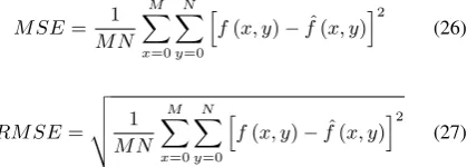
DsH(w) = sgn(w) max (0;|w| −T) (22)

Semi-soft Thresholding

DSST T1(w) =  



0 |w| ≤T

sgn(w)T1(|_T1−w|−_TT) T <|w| ≤T1

w |w|> T1

(23)

(5) After modifying the wavelet coefficients in the subbands take the inverse transform to reconstruct the image. (6) Compute the inverse variance stabilization transform of the

above reconstructed image to get denoised image which is an estimation of the original one.

Many shrinkage rules are associated with the wavelet process-ing. The threshold may be calculated globally, level dependent or subband dependent. But here we are calculating the threshold globally.

Table 1. Double Density Dual Tree First stage Wavelet filter Coefficients (Tree 1)

h0(−n) h1(−n) h2(−n)

0 0 0

0.00069616789827 -0.00014203017443 0.00014203017443 -0.02692519074183 0.00549320005590 -0.00549320005590 -0.04145457368920 0.01098019299363 -0.00927404236573 0.19056483888763 -0.13644909765612 0.07046152309968 0.58422553883167 -0.21696226276259 0.13542356651691 0.58422553883167 0.33707999754362 -0.64578354990472 0.19056483888763 0.33707999754362 0.64578354990472 -0.04145457368920 -0.21696226276259 -0.13542356651691 -0.02692519074183 -0.13644909765612 -0.07046152309968 0.00069616789827 0.01098019299363 0.00927404236573 0 0.00549320005590 0.00549320005590 0 -0.00014203017443 -0.00014203017443

0 0 0

Table 2. Double Density Dual Tree First stage Wavelet filter Coefficients (Tree 2)

g0(−n) g1(−n) g2(−n)

0 0 0

0 0 0

Apply the Forward Transform (DWT/UDWT/ DTCWT/Double density) Apply the Forward Transform (DWT/UDWT/ DTCWT/Double density) Apply Wavelet Shrinkage Apply Wavelet Shrinkage Apply the Inverse Transform (DWT/UDWT/ DTCWT/double density) Apply the Inverse Transform (DWT/UDWT/ DTCWT/double density) Image Corrupted with noise Image Corrupted with noise Denoised Image Denoised Image Apply VST Transform Square Root/ Freeman & Tukey/ Anscombe Apply VST Transform Square Root/ Freeman & Tukey/ Anscombe Apply Inverse VST Transform Square Root/ Freeman & Tukey/ Anscombe Apply Inverse VST Transform Square Root/ Freeman & Tukey/ Anscombe

Fig. 6. Denoising system using Multiscale Transform

The above filters are the first stage filters in the tree 1 and tree 2 of double density dual tree discrete wavelet transform. These filters are only applied in the first stage decomposition only. The filters for the remaining stages are given below.

Table 3. Double Density Dual Tree Wavelet filter Coefficients from second stage onwards (Tree 1) h0(−n) h1(−n) h2(−n)

0.00017870679071 -0.00012344587034 0.00001437252392 -0.02488304194507 0.01718853971559 -0.00200122286479 0.00737700819766 -0.00675291099550 0.00027261232228 0.29533805776119 0.02671809818132 0.06840460220387 0.59529279993637 -0.64763513288874 0.01936710587994 0.45630440337458 0.47089724990858 -0.68031992557818 0.11239376309619 0.16040017815754 0.42976785708978 -0.01971220693439 -0.01484700537727 0.11428688385011 -0.00813549683439 -0.00588868840296 0.05057805218407 0.00005956893024 0.00004311757177 -0.00037033761102

Table 4. Double Density Dual Tree Wavelet filter Coefficients from second stage onwards (Tree 2) g0(−n) g1(−n) g2(−n)

0.00005956893024 0.00004311757177 -0.00037033761102 -0.00813549683439 -0.00588868840296 0.05057805218407 -0.01971220693439 -0.01484700537727 0.11428688385011 0.11239376309619 0.16040017815754 0.42976785708978 0.45630440337458 0.47089724990858 -0.68031992557818 0.59529279993637 -0.64763513288874 0.01936710587994 0.29533805776119 0.02671809818132 0.06840460220387 0.00737700819766 -0.00675291099550 0.00027261232228 -0.02488304194507 0.01718853971559 -0.00200122286479 0.00017870679071 -0.00012344587034 0.00001437252392

4. EVALUATION CRITERIA FOR DENOISING ALGORITHMS

To evaluate the quality of the image processing algorithms there are several metrics proposed in the literature. The metrics are classified as pixel difference based measures, correlation based measures, edge based measures, spectral distance measures, con-text based measures and Human visual system based measures. Here we are comparing our denoising algorithms using a group of metrics drawn from the above class and performance of the algorithms was observed.

4.1 Pixel difference based measures

4.1.1 Minkowski metrics. TheLγnorm of the dissimilarity of

two images can be calculated by calculating the minkowski av-erage of the pixel differences spatially and then chromatically as given below

εγ₌ 1

K K X k=1 ( 1 M N M−1 X x=0 N−1 X x,y=0

fk(x, y)− ˆ

fk(x, y) γ) 1 γ (24)

Wheref(x, y) is the reference image,fˆ(x, y) is the estimated image of f(x, y) by our denoising algorithm with the input g(x, y)which is a noisy version off(x, y). Forγ= 1we obtain the absolute difference (AD), forγ= 2we will obtain the mean square error (MSE). Along with these two measures we are cal-culating minkowski measures forγ= 3andγ= 4in this paper to observe the performance of our algorithms.

4.1.2 PSNR (Peak Signal to Noise Ratio). PSNR is the peak signal-to-noise ratio in decibels (dB). The PSNR is only mean-ingful for data encoded in terms of bits per sample, or bits per pixel. For example, an image with 8 bits per pixel contains inte-gers from 0 to 255.

P SN R= 20log10

2B₋₁ √

M SE

(25)

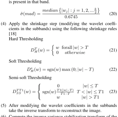
Where B represents bits per sample and MSE (Mean Squared error) is the mean square error between a signalf(x, y)and an approximationfˆ(x, y)is the squared norm of the difference di-vided by the number of elements in the signal.

M SE= 1

M N M X x=0 N X y=0 h

f(x, y)−_fˆ_{(x, y)}i2 ₍₂₆₎

RM SE= v u u t 1 M N M X x=0 N X y=0 h

f(x, y)−fˆ(x, y)i2 (27)

MSE and RMSE measures the difference between the original and distorted sequences. PSNR measures the fidelity i.e how close a sequence is similar to an original one.

4.1.3 Maximum Difference. Maximum difference is defined as M D= max

f(x, y)− ˆ

f(x, y)

(28)

The large value of maximum difference means denoised image is poor quality.

4.1.4 Normalised Absolute Error (NAE). The large value of normalised absolute error means that denoised image is poor quality and is defined as

N AE=

M−1 P x=0 N−1 P y=0

f(x, y)− ˆ

f(x, y) M−1 P x=0 N−1 P y=0

|f(x, y)|

(29)

4.1.5 Signal to Noise Ratio (SNR). Signal to noise ratio in an image is calculated as

SN R=µ

σ

4.2 Correlation based measures

The correlation between two images can also be quantified in-terms of correlation function. These measures measure the simi-larity between the two images hence in this sense they are com-plementary to the difference based measures.

4.2.1 Structural content. For anM×N image the structural content is defined as

SC= 1

K K X k=1 M−1 P x=0 N−1 P y=0

fk(x, y)2

M−1 P x=0 N−1 P y=0 ˆ

fk(x, y)2

(30)

4.2.2 Normalised cross correlation measure (NK). The nor-malised cross correlation measure is defined as

N K= 1

K K X k=1 M−1 P x=0 N−1 P y=0

fk(x, y) ˆfk(x, y)

M−1 P x=0 N−1 P y=0

fk(x, y)2

(31)

4.3 HVS based metrics

4.3.1 Universal Image Quality Index (UQI). It is a measure used to find the image distortion. It is mathematically defined by making the image distortion relative to the reference image as a combination of three factors: Loss of correlation, Lumi-nance distortion and contrast distortion. If two imagesf(x, y)

andfˆ(x, y)are considered as a matrices with M column and N rows containing pixel valuesf(x, y)andfˆ(x, y)respectively the universal image quality index Q may be calculated as a prod-uct of three components

Q= σffˆ

σfσfˆ

· 2 ¯f¯ˆf

f2_{+ ˆf}2 ·

2σfσfˆ σ2

f+σ2_fˆ

(32)

Where f¯ = 1

M N M−1 P x=0 N−1 P y=0

f(x, y) and

¯

ˆf = 1

M N M−1 P x=0 N−1 P y=0 ˆ

f(x, y) σ_ffˆ =

1

M+N−1

M−1 P x=0 N−1 P y=0

f(x, y)−_f¯_ˆ

f(x, y)−¯_ˆf

σ2

f =

1

M+N−1

M−1 P x=0 N−1 P y=0

f(x, y)−f¯

2 and σ2 ˆ f = 1

M+N−1

M−1 P x=0 N−1 P y=0 ˆ

f(x, y)−¯ˆf 2

The first component is the correlation coefficient which mea-sures the degree of linear correlation between images. It varies in the range [-1,1]. The best value 1 is obtained when the images are linearly related. The second component measures how close the mean luminance is between images with a range [0, 1]. The third component measures the contrasts of the images the value range for this component is [0, 1]. The range of values for Q is [-1, 1]. The best value 1 is achieved if and only if the images are identical.

4.3.2 Structural similarity (SSIM) index. Structural similarity (SSIM) index is a method for measuring the similarity between two images [28]. The SSIM index is a full reference metric, in other words, the measuring of image quality based on an ini-tial uncompressed or distortion-free image as reference. SSIM is designed to improve on traditional methods like peak signal-to-noise ratio (PSNR) and mean squared error (MSE), which have proved to be inconsistent with human eye perception. The SSIM metric is calculated on various windows of an image. The

mea-sure between two windows x and y of common size NN is [19]:

SSIM(x, y) = (2µxµy+c1) (2σxy+c2)

µ2

x+µ2y+c1

σ2

x+σy2+c2

(33)

5. RESULTS & CONCLUSIONS

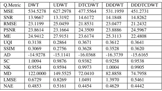
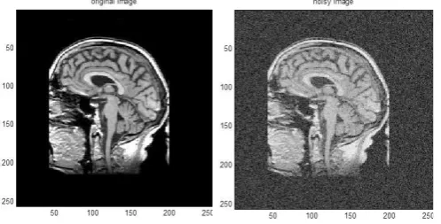
The performance of the algorithms was evaluated based on the above quality metrics obtained from the original image and the denoised image. The X-ray image was corrupted with Poisson noise. The noise variance here is dependent on the data present in the image. The brain image acquired under low intensity levels is corrupted with Rician noise with sigma=20. The algorithms designed are applied on these two images and performances of the algorithms are evaluated using the above metrics.

The results show that the denoising using discrete wavelet transform is denoising the images but it fails to preserve the edges with orientation because of its shift variance nature. The undecimated wavelet transform will overcome this drawback in little amount with the expense of high computational cost. So we used the dual tree complex transforms and double density complex wavelet transforms to overcome this drawbacks and to reduce the computational cost. The denoised images by these transforms are preserving the edge information excellently than the discrete wavelet transforms. Here we used the universal threshold for all the subbands in the image. The performance of the algorithms can be improved using subband dependent and level dependent thresholds in place of universal threshold used in our work.

Table 5. VST:Anscombe, Noise:Poisson

Q.Metric DWT UDWT DTCDWT DDDWT DDDTCDWT MSE 8.8750 4.8179 4.6285 5.4525 4.7981 SNR 33.6655 36.3168 36.4922 35.7759 36.3324 RMSE 2.9791 2.1950 2.1514 2.3351 2.1905 PSNR 40.3375 42.2906 43.1648 42.4533 43.2085 ME 4.3967 3.0643 2.9760 3.1915 2.9733 UQI 0.3216 0.3763 0.3858 0.3516 0.3590 SSIM 0.9328 0.9579 0.9609 0.9614 0.9633 AD -0.0679 -0.0588 -0.0659 -0.0239 -0.0375 SC 0.9999 1.0007 1.0002 1.0023 1.0017 NK 0.9996 0.9994 0.9997 0.9986 0.9989 MD 46.4963 30.6751 34.2788 30.4080 28.7097 LMSE 0.8060 0.4465 0.3945 0.3662 0.3562 NAE 0.0226 0.0177 0.0177 0.0189 0.0179

Table 6. VST:Anscombe, Noise:Rician

Fig. 7. a) Original Image b) Noisy Image

Fig. 8. a) Denoised using DWT b) Denoised using UDWT

Fig. 9. a) Denoised using DTCDWT b) Denoised using DDDTCDWT

Fig. 10. a) Original Image b) Noisy Image

Fig. 11. a) Denoised using DWT b) Denoised using UDWT

Fig. 12. a) Denoised using DTCDWT b) Denoised using DDDTCDWT

6. REFERENCES

[1] J.W. Goodman, ”Some fundamental properties of speckle,” J. Opt. Soc. Am., vol. 66, no. 11, pp. 1145-1149, 1976. [2] C.B. Burckhardt, ”Speckle in ultrasound B-mode scans,”

IEEE Trans. Sonics Ultrasonics, vol. SU-25, no. 1, pp. 1-6, 1978.

[3] Z. Tao, H. D. Tagare, and J. D. Beaty. Evaluation of four probability distribution models for speckle in clinical car-diac ultrasound images. IEEE Transactions on Medical Imaging, 25(11):14831491, 2006.

[4] P. C. Tay, S. T. Acton, and J. A. Hossack. A stochastic ap-proach to ultrasound despeckling. In Biomedical Imaging: Nano to Macro, 2006. 3rd IEEE International Symposium on, pages 221224, 2006.

[5] J.S. Lee, ”Digital image enhancement and noise filtering by using local statistics,” IEEE Trans. Pattern Anal. Mach. Intell., PAMI-2, no. 2, pp. 165-168, 1980.

[6] J.S. Lee, ”Speckle analysis and smoothing of synthetic aperture radar images,” Comp. Graphics Image Process., vol. 17, pp. 24-32, 1981.

[7] J.S. Lee, ”Refined filtering of image noise using local statistics,” Comput. Graphics Image Process, vol. 15, pp. 380-389, 1981.

[8] V.S. Frost, J.A. Stiles, K.S. Shanmungan, and J.C. Holtz-man, ”A model for radar images and its application for adaptive digital filtering of multiplicative noise,” IEEE Trans. Pattern Anal. Mach. Intell., vol. 4, no. 2, pp. 157-165, 1982.

[10] D.T. Kuan, A.A. Sawchuk, T.C. Strand, and P. Chavel, ”Adaptive restoration of images with speckle,” IEEE Trans. Acoust., vol. ASSP-35, pp. 373-383, 1987, doi:10.1109/TASSP.1987.1165131.

[11] J. Saniie, T. Wang, and N. Bilgutay, ”Analysis of homo-morphic processing for ultrasonic grain signal characteri-zation,” IEEE Trans. Ultrason. Ferroelectr. Freq. Control, vol. 3, pp. 365-375, 1989, doi:10.1109/58.19177.

[12] A. Pizurica, A. M.Wink, E. Vansteenkiste, W. Philips, and J. Roerdink, ”A review of wavelet denoising in mri and ul-trasound brain imaging,” Curr. Med. Imag. Rev., vol. 2, no. 2, pp. 247-260, 2006.

[13] D.L. Donoho, ”Denoising by soft thresholding,” IEEE Trans. Inform. Theory, vol. 41, pp. 613-627, 1995. [14] X. Zong, A. Laine, and E. Geiser, ”Speckle reduction and

contrast enhancement of echocardiograms via multiscale nonlinear processing,” IEEE Trans. Med. Imaging, vol. 17, no. 4, pp. 532-540, 1998.

[15] Paul Butler, ”Applied Radiological Imaging for Medical Students”, Ist Edition, Cambridge University Press, 2007. [16] Rangaraj M. Rangayyan, ”Biomedical Signal Analysis A

Case study Approach”, IEEE Press, 2005.

[17] Stephane Mallat, ”A Wavelet Tour of signal Processing”, Elsevier, 2006.

[18] D L Donoho and M. Jhonstone, ”Wavelet shrinkage: Asymptopia? ”, J.Roy.Stat.Soc., SerB, Vol.57, pp. 301-369, 1995.

[19] Z. Wang, A. C. Bovik, H. R. Sheikh and E. P. Simoncelli, ”Image quality assessment: From error visibility to struc-tural similarity,” IEEE Transactions on Image Processing, vol. 13, no. 4, pp. 600-612, Apr. 2004.

[20] Ivan W.Selesnick, Richard G.Baraniuk, Nick G. Kingsbury, ”The Dual Tree Complex Wavelet Transform”, IEEE Sig-nal Processing Magazine, November 2005.

[21] I. W. Selesnick, ”The design of Hilbert transform pairs of wavelet bases via the flat delay filter,” in Proc. IEEE Int. Conf. Acoust., Speech, Signal Process., May 2001. [22] N. G. Kingsbury, ”The dual-tree complex wavelet

trans-form: A new technique for shift invariance and directional filters,” in Proc. Eighth IEEE DSP Workshop, Salt Lake City, UT, Aug. 9-12, 1998.