2018 International Conference on Computer, Electronic Information and Communications (CEIC 2018) ISBN: 978-1-60595-557-5
A Robust Joint Estimation Method of Time Delay and Doppler
Frequency Shift
Ling YU
1,*, Fang-lin NIU
1and Jin-feng ZHANG
21
School of Electronic & Information Engineering, Liaoning University of Technology, Jinzhou 121001, China
2
Shenzhen Key Lab of Advanced Communications and Information Processing, Shenzhen University, Shenzhen 518060, China
*Corresponding author
Keywords: Alpha-stable distribution, Cyclic ambiguity function, Doppler frequency shift, Sigmoid transform, Time delay.
Abstract. In this paper, a novel concept, the Sigmoid transform based cyclic correlation, is proposed and a relative estimator named the Sigmoid transform based cyclic cross-ambiguity function is also derived to handle the joint estimation problem in the presence of impulsive noise and co-channel interference. Based on these definitions, a novel joint estimation method of the time delay and the Doppler frequency shift is proposed. Simulations have verified its superior performances over existing methods based on cyclic ambiguity function or generalized fractional lower-order cyclic cross-ambiguity function, especially under impulsive noise. Meanwhile, it is more applicable for practical applications since it is parameter-free.
Introduction
During the past decades, specialists and scholars have made huge contributions to the research on the cross ambiguity function (CAF) [1-3], especially in the presence of Gaussian noise. A linear canonical transform was introduced to ambiguity function for the time-frequency analysis of the cubic phase signal in [4]. A generalized Wigner–Ville distribution (WDL)was combined with CAF in [5]. However, these methods are derived upon the second-order statistics, which leads to their deterioration under impulsive noise environment. To better the solution, a full set of novel concepts and methods are proposed and developed after the proposal of the fractional lower order statistics by Nikias and the fractional lower order statistics based ambiguity function[6; 7](FLOSAF) is one of the methods. FLOSAF works well under both Gaussian and non-Gaussian noises, but its performances deteriorates in the presence of co-channel interference. On the other hand, although cyclic ambiguity function (CCA) proposed in [8] could handle the co-channel interference, it is still a second-order statistics based method. Meanwhile, it deteriorates under impulsive noise undoubtedly. During the search for a better method which considers both Non-Gaussian noise model and co-channel interference, the fractional lower-order cyclic cross-ambiguity function (FCCA) and the generalized fractional lower-order cyclic cross-ambiguity function algorithm (GFCCA) are presented in [9]. However, they still have their own shortcomings. For instance, these two methods are based on the fractional lower-order statistics (FLOS), which leads to their reliance on the a priori knowledge of
impulsive noise during the choices of the order parameters a and b. Moreover, the performance of
FLOS-based methods will degrade under highly impulsive noise. Therefore, a void still remains in the search for a novel method with better robustness in the presence of both non-Gaussian noise and co-channel interference.
superiority over existing methods under both non-Gaussiannoise and co-channel interference. In this paper, the non-Gaussian noise is modeled by alpha-stable distribution[10].
Background Signal Model
Suppose two received signals x t
( )
and y t( )
as( )
( )
1( )
i( )
x t =s t +w t +s t (1)
( )
(
)
j2π( )
( )
2
d f t
i
y t =s t−D e− +w t +s t (2)
wheres t
( )
denotes the signal of interest and it is a cyclostationary signal. D denotes the time delaybetween the receivers. fddenotes the Doppler frequency shift caused by the relative moving between
the receiver and the object.s ti
( )
denotes the co-channel interference modulated with the same carrierfrequency with s t
( )
. w t1( )
and w t2( )
denote additive noises which obey alpha-stabledistribution[11]. As a direct generalization of the Gaussian distribution, the alpha-stable distribution
is completely determined by four parameters: the characteristic exponent
α
, the symmetric parameterβ, the location parameter µ and the dispersion parameter γ .
SigmoidCCA
Sigmoid transform is a commonly used nonlinear transform[12-14]. Its definition is shown in Eq.(3).
( )
( )
2
Sigmoid 1
1 exp
x t
x t
= −
+ − (3)
For complex Z t
( )
= X t( )
+jY t( )
,( )
( )
(
)
(
(
( )
)
(
( )
)
)
2
Sigmoid 1
1 exp cos jsin
Z t
X t Y t Y t
= −
+ − − + − (4)
A novel cyclic correlationRx,Sigmoid
( )
ετ referred to as Sigmoid transform based cyclic correlation
(SigmoidCC) is defined in Eq.(5),
( )
(
)
(
)
2
* j2π
,Sigmoid
2 1
= lim Sigmoid 2 Sigmoid 2 e d
T
t x
T T
R x t x t t
T
ε τ τ τ − ε
→∞ −
+ −
∫
(5)For a finite duration signal, Rxε,Sigmoid
( )
τ could be estimated by Eq.(6).( )
(
)
(
)
2
* j2π
,Sigmoid
2 1
ˆ = Sigmoid 2 Sigmoid 2 e d
T
t x
T
R x t x t t
T
ε ε
τ τ τ −
−
+ −
∫
(6)Sigmoid transform based cyclic cross-correlation Ryxε ,Sigmoid
( )
τ is given inEq.(7).( )
(
)
(
)
2
* j2π
,Sigmoid
2 1
= lim Sigmoid 2 Sigmoid 2 e d
T
t
yx T
T
R x t y t t
T
ε ε
τ τ τ −
→∞ −
+ −
( )
(
)
(
)
2
* j2π
,Sigmoid
2 1
ˆ = Sigmoid 2 Sigmoid 2 e d
T
t yx
T
R x t y t t
T
ε ε
τ τ τ −
−
+ −
∫
(8)A novel cyclic ambiguity functionCyxε,Sigmoid
(
u f,)
, named Sigmoid transform based cycliccross-ambiguity function (SigmoidCCA), is shown in Eq.(9).
(
)
(
)
( )
* jπ,Sigmoid , = ,Sigmoid ,Sigmoid e d
f f
yx x yx
Cε u f Rε τ u Rε− τ − τ τ
+
∫
(9)And the joint estimation method based on SigmoidCCA is shown in Eq.(10)
(
D fˆ , ˆd)
argmaxCyx,Sigmoid(
u f,)
ε= (10)
Simulation
Simulation conditions:The signal of interest is set as a BPSK signal with the carrier frequency
0.5
c s
f = f and thebaud rate ad1=0.2fs, where fs is the sampling frequency. Time delay is set as 16
sample intervals and theDoppler frequency shift (DFS) is set as 0.3125 fs . The co-channel
interference is another BPSK signal with the same carrier frequency but a different baud
ratead2=0.6fs. The signal to interference ratio (SIO) is 0dB. The additional noises are SαS noises
with µ=0. The generalized signal-to-noise ratio (GSNR) is employed to measure the noise intensity,
and it is defined in Eq.(11)
2 10
GSNR=10 log (σs /γw) (dB) (11)
where 2
s
σ is the signal variance and γ is the dispersion parameter of SαS noise. The estimation
accuracyPais defined in Eq.(12), where Vˆ is the estimation value and V is the true one.
ˆ
1 100%
a
V V P
V
−
= − ×
(12)
In order to verify the superior performances of SigmoidCCA over existing methods such as CCA, FCCA and GFCCA, simulation experiments are carried out as follows. And the order parameters for
FCCA and GFCCA are a=b=0.1. The results in Simulations 2 and 3 are based on 500 Monte-Carlo
simulations.
Simulation 1: CCA, FCCA, GFCCA and SigmoidCCA for a single estimation
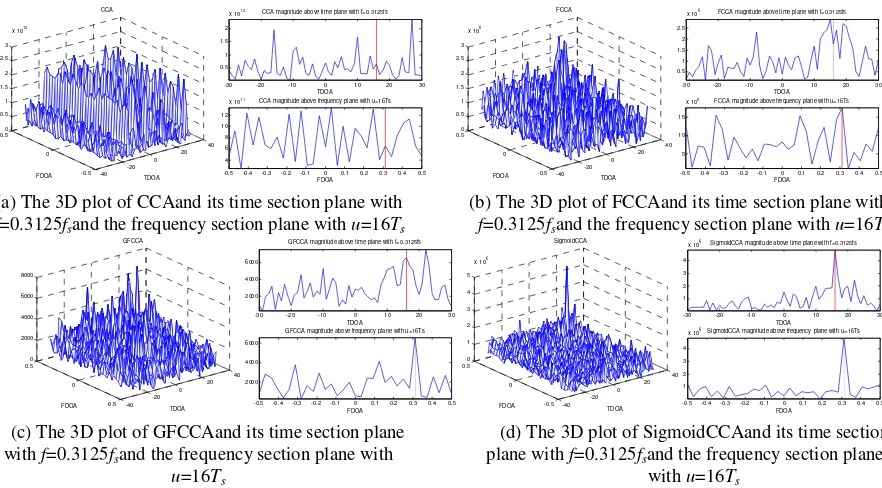
Simulation 1 shows the estimation results of CCA, FCCA, GFCCA and SigmoidCCAfor a single
trial of data under bothSαS noise and co-channel interference. In Figure 1, the red solid line denotes
-40 -20 0 20 40 -0.5 0 0.5 0 0.5 1 1.5 2 2.5 3
x 1012
TDOA CCA
FDOA
-30 -20 -10 0 10 20 30 0.5
1 1.5 2
x 1012 CCA magnitude above time plane with f=0.3125fs
TDOA
-0.5 -0.4 -0.3 -0.2 -0.1 0 0.1 0.2 0.3 0.4 0.5 4
6 8 10 12
x 1011 CCA magnitude above frequency plane with u=16Ts
FDOA -40 -20 0 20 40 -0.5 0 0.5 0 0.5 1 1.5 2 2.5 3
x 106
TDOA FCCA
FDOA
-30 -20 -10 0 10 20 30 0.5
1 1.5 2 2.5
x 106 FCCA magnitude above time plane with f=0.3125fs
TDOA
-0.5 -0.4 -0.3 -0.2 -0.1 0 0.1 0.2 0.3 0.4 0.5 5
10 15
x 105 FCCA magnitude above frequency plane with u=16Ts
FDOA
(a) The 3D plot of CCAand its time section plane with (b) The 3D plot of FCCAand its time section plane with
f=0.3125fsand the frequency section plane with u=16Ts f=0.3125fsand the frequency section plane with u=16Ts
-40 -20 0 20 40 -0.5 0 0.5 0 2000 4000 6000 8000 TDOA GFCCA FDOA
-30 -20 -10 0 10 20 30 2000
4000 6000
GFCCA magnitude above time plane with f=0.3125fs
TDOA
-0.5 -0.4 -0.3 -0.2 -0.1 0 0.1 0.2 0.3 0.4 0.5 2000
4000 6000
GFCCA magnitude above frequency plane with u=16Ts
FDOA -40 -20 0 20 40 -0.5 0 0.5 0 1 2 3 4 5
x 106
TDOA SigmoidCCA
FDOA
-30 -20 -10 0 10 20 30 1
2 3 4
x 106 SigmoidCCA magnitude above time plane with f=0.3125fs
TDOA
-0.5 -0.4 -0.3 -0.2 -0.1 0 0.1 0.2 0.3 0.4 0.5 1
2 3 4
x 106SigmoidCCA magnitude above frequency plane with u=16Ts
FDOA
(c) The 3D plot of GFCCAand its time section plane with f=0.3125fsand the frequency section plane with
u=16Ts
(d) The 3D plot of SigmoidCCAand its time section plane with f=0.3125fsand the frequency section plane
[image:4.612.85.526.66.310.2]with u=16Ts
Figure 1. The estimation results of CCA, FCCA, GFCCA and SigmoidCCAunder co-channel interference (SIO=0dB) and impulsive noise (GSNR=0dB,α =1).
In Figure 1, CCA fails when impulsive noise is presented. GFCCA also fails under intensive
impulsive noise as α=1. On contrast, SigmoidCCA has clear peaks. Meanwhile, cyclostationary
theory is utilized in all the methods, which keeps 3D plotsfrom wrong peaks caused by co-channel interference and verifies their robustness for co-channel interference.
Simulation 2: estimation accuracy versus GSNR
From Figure 2, when GSNR is higher than 10dB, the four methods all work well under weak impulsive noise. CCAdeteriorates quickly when GSNR decreases. SigmoidCCA outperforms other methods when GSNR is extremely low.
-5 0 5 10 15
0 20 40 60 80 100 GSNR(dB) A cc u ra cy ( % )
Doppler frequency shift
CCA FCCA GFCCA SigmoidCCA
-5 0 5 10 15
0 20 40 60 80 100 GSNR(dB) A cc u ra cy ( % ) delay CCA FCCA GFCCA SigmoidCCA
Figure 2. Estimation accuracy versus GSNR(α =1.5).
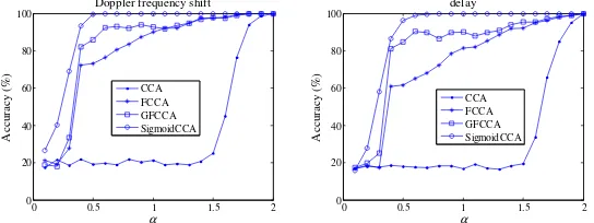
Simulation 3: estimation accuracy versus characteristic exponentα( GSNR=0dB)
Simulation 3 is the comparison among four methods when GSNR=0dB and the results are shown
in Figure 3. Similar to Simulation 2, all these methods perform well ifnoise obeys Gaussian
distribution whenα =2. On the other hand, when the noise becomes more impulsive, for example
[image:4.612.164.441.457.559.2]0 0.5 1 1.5 2 0
20 40 60 80 100
α
A
cc
u
ra
cy
(
%
)
Doppler frequency shift
CCA FCCA GFCCA SigmoidCCA
0 0.5 1 1.5 2
0 20 40 60 80 100
α
A
cc
u
ra
cy
(
%
)
delay
[image:5.612.167.439.69.171.2]CCA FCCA GFCCA SigmoidCCA
Figure 3. Estimation accuracy versus α.
Conclusion
In this paper, a novel concept named Sigmoid transform based cyclic correlation (SigmoidCC) is first proposed. Then a robust estimator termed Sigmoid transform based cyclic cross-ambiguity function(SigmoidCCA) is derived upon SigmoidCC to handle the time delay and Doppler frequency shift problem in the presence of impulsive noise and co-channel interference. Theoretical analysis and simulation results show that SigmoidCCA has better estimation precision than the others, such as CCA, FCCA and GFCCA methods, even when GSNR is extremely low or when the impulsiveness is intensive.
Acknowledgments
This work is partly supported by National Natural Science Foundation of China (61139001, 61172108 and 61501301), Fundamental Research Funds for the Universities of Liaoning Educational Committee (JQL201715405), and Natural Science Foundation of Liaoning Province of China(201602373).
References
[1] X. F. Song, P. Willett, and S. L. Zhou. Range Bias Modeling for
Hyperbolic-Frequency-Modulated Waveforms in Target Tracking, IEEE Journal of Oceanic Engineering 37.4 (2012): 670-679.
[2] Y. Z. Li, S. A. Vorobyov, and V. Koivunen. Ambiguity Function of the Transmit
Beamspace-Based Mimo Radar, IEEE Transactions on Signal Processing63.17 (2015): 4445-4457.
[3] J. Wu, et al. On the Feasibility of Ionosphere-Modeled Satellite Positioning by a Hierarchical
Ambiguity Function Methodology, Journal of the Chinese Institute of Engineers 38.8 (2015):
1002-1009.
[4] R. Tao, et al. Ambiguity Function Based on the Linear Canonical Transform, IET Signal
Processing6.6 (2012): 568-576.
[5] Z. C. Zhang. Unified Wigner–Ville Distribution and Ambiguity Function in the Linear Canonical
Transform Domain, Signal Processing114.C (2015): 45-60.
[6] X. Y. Ma, and C. L. Nikias. Joint Estimation of Time Delay and Frequency Delay in Impulsive
Noise Using Fractional Lower Order Statistics, IEEE Transactions on Signal Processing 44.11
(1996): 2669-2687.
[8] Z. T. Huang, et al. Joint Estimation of Doppler and Time-Difference-of-Arrival Exploiting
Cyclostationary Property, IEE Proceedings - Radar, Sonar and Navigation149.4 (2002): 161-165.
[9] Y. Liu, T. S. Qiu, and J. C. Li. Joint Estimation of Time Difference of Arrival and Frequency Difference of Arrival for Cyclostationary Signals under Impulsive Noise, Digital Signal Processing 46.C (2015): 68-80.
[10] M. Shao, and C. L. Nikias. Signal Processing with Fractional Lower Order Moments: Stable
Processes and Their Applications, Proceedings of the IEEE81.7 (1993): 986-1010.
[11] C. L. Nikias, and M. Shao. Signal Processing with Alpha-Stable Distributions and Applications.
USA: Wiley-Interscience, 1995. Print.
[12] K. H. Brodersen, et al. Variational Bayesian Mixed-Effects Inference for Classification Studies,
Neuroimage76.1 (2013): 345-361.
[13] N. Saini, and A. Sinha. Face and Palmprint Multimodal Biometric Systems Using Gabor–Wigner
Transform as Feature Extraction, Pattern Analysis and Applications18.4 (2015): 921-932.
[14] H. T. Lang, et al. Ship Classification in Sar Image by Joint Feature and Classifier Selection, IEEE