Parallel LQP alternating direction method for solving variational inequality problems with separable structure

R E S E A R C H

Open Access

Parallel LQP alternating direction method for

solving variational inequality problems with

separable structure

Abdellah Bnouhachem

_{and Abdelouahed Hamdi}

Dedicated to Professor Shih-Sen Chang on the occasion of his 80th birthday.

*_{Correspondence:}

[email protected] 3_{Department of Mathematics,}

Statistics and Physics, College of Arts and Sciences, Qatar University, P.O. Box 2713, Doha, Qatar Full list of author information is available at the end of the article

Abstract

In this paper, we propose a logarithmic-quadratic proximal alternating direction method for structured variational inequalities. The predictor is obtained by solving series of related systems of nonlinear equations, and the new iterate is obtained by a convex combination of the previous point and the one generated by a

projection-type method along a new descent direction. Global convergence of the new method is proved under certain assumptions. Preliminary numerical

experiments are included to verify the theoretical assertions of the proposed method.

MSC: 90C33; 49J40

Keywords: variational inequalities; monotone operator; logarithmic-quadratic proximal method; projection method; alternating direction method

1 Introduction

The problem we are concerned with in this paper is for the following variational inequal-ities: findu∈such that

u–uTF(u)≥, ∀u∈, (.)

with

u=

x y

, F(u) =

f(x)

g(y)

and

=(x,y)|x∈Rn₊,y∈Rm₊,Ax+By=b,

(.)

whereA∈Rl×n,B∈Rl×mare given matrices,b∈Rlis a given vector, andf :Rn₊→Rn,

g:Rm

+ →Rm are given monotone operators. Studies and applications of such problems

can be found in [–]. By attaching a Lagrange multiplier vectorλ∈Rl _{to the linear} constraintAx+By=b, problem (.)-(.) can be explained in terms of findingw∈W

such that

w–wTQ(w)≥, ∀w∈W, (.)

where

w=

⎛ ⎜ ⎝

x y λ

⎞ ⎟

⎠, Q(w) =

⎛ ⎜ ⎝

f(x) –AT_λ g(y) –BTλ Ax+By–b

⎞ ⎟

⎠, W=Rn₊×Rm₊ ×Rl. (.)

Problem (.)-(.) is referred to as SVI (structured variational inequalities).

The alternating direction method (ADM) is a powerful method for solving the struc-tured problem (.)-(.), since it decomposes the original problems into a series of sub-problems with a lower scale, originally proposed by Gabay and Mercier [] and Gabay []. The classical proximal alternating direction method (PADM) [–] is an effective numerical approach for solving variational inequalities with separable structure. In [], He proposed splitting augmented Lagrangian methods for structured monotone varia-tional inequalities whose operator is composed by two separable operators. For given (xk_,yk_,λk_)∈Rn

++×Rm++×Rl, the predictorw˜k= (x˜k,y˜k,λ˜k) is obtained via the following

steps:

Step . Solve the following variational inequality to obtainx˜k_:

x–x˜kTfx˜k–ATλk–HAx˜k+Byk–b≥, ∀x∈Rn₊₊. (.)

Step . Solve the following variational inequality to obtainy˜k_:

y–y˜kTg˜yk–BTλk–HAxk+By˜k–b≥, ∀y∈Rm₊₊. (.)

Step . Updateλkvia

˜

λk=λk–HAx˜k+By˜k–b. (.)

The main advantage of the method of [] is that the predictor is obtained by solving subproblems in a parallel wise. Recently, Yuan and Li [] have developed a logarithmic quadratic proximal (LQP)-based decomposition method by applying the LQP terms to regularize the ADM subproblems. The new iterative (xk+_,yk+_,λk+_{) in [] is obtained via}

the following procedure: From a givenwk= (xk,yk,λk)∈Rn₊₊×Rm₊₊×Rl, andμ∈(, ), (xk+_,yk+_,λk+_{) is obtained via solving the following system:}

f(x) –ATλk–HAx+Byk–b+Rx–xk+μxk–X_kx–= ,

g(y) –BT_λk_–HAxk+_{+By–b+Sy–y}k_+μyk_–Y ky–

= ,

λk+=λk–HAxk+Byk–b,

In the present paper, inspired by the above cited works and by the recent works go-ing in this direction, we proposed a new LQP-based prediction-correction method. The predictor is obtained by using the idea of He [] to solve series of related systems of non-linear equations, and the new iterate is obtained by a convex combination of the previous point and the one generated by a projection-type method along another descent direction. Under certain conditions, we proved the global convergence of the proposed algorithm. Preliminary numerical experiments are included to verify the theoretical assertions of the proposed method.

2 The proposed method

In this section, we recall some basic definitions and properties, which will be frequently used in our later analysis. Some useful results proved already in the literature are also summarized. The first lemma provides some basic properties of projection onto.

Lemma . Let G be a symmetric positive definite matrix andbe a nonempty closed convex subset of Rl_{,we denote P}

,G[·]as the projection under the G-norm,i.e.,

P,G[v] =argmin

v–uG|u∈

.

Then,we have the following inequalities:

z–P,G[z]

T

GP,G[z] –v

≥, ∀z∈Rl,v∈; (.)

P,G[u] –P,G[v]_G≤ u–vG, ∀u,v∈Rl; (.)

_u–P,G[z]

G≤ z–u 

G–z–P,G[z] 

G, ∀z∈R

l_{,u∈. (.)}

In course, we always make the following standard assumptions:

Assumption A f is monotone with respect toRn₊₊ andg is monotone with respect to

Rm ++.

Assumption B The solution set of SVI, denoted byW∗, is nonempty.

Now, we suggest and consider the new LQP alternating direction method (LQP-ADM) for solving SVI as follows.

Prediction step: For a givenwk_{= (x}k_,yk_,λk_)∈Rn

++×Rm++×Rl, andμ∈(, ), the

pre-dictorw˜k_{= (x˜}k_,y˜k_,λ˜k_)∈Rn

++×Rm++×Rlis obtained via solving the following system:

f(x) –ATλk–HAx+Byk–b+Rx–xk+μxk–X_kx–= , (.a)

g(y) –BTλk–HAxk+By–b+Sy–yk+μyk–Y_ky–= , (.b)

˜

λk=λk–HAx˜k_+B˜yk_{–b. (.c)}

Correction step: The new iteratewk+_(α

k) = (xk+,yk+,λk+) is given by

wk+(αk) = ( –σ)wk+σPW

wk–αkG–d

where

αk= ϕk

wk_–w˜k G

, (.)

ϕk:=wk–w˜kM+

λk–λ˜kTAxk–x˜k+Byk–y˜k, (.)

dwk,w˜k=

⎛ ⎜ ⎝

f(x˜k_{) –A}T_λ˜k_+AT_H(A(xk_–x˜k_{) +B(y}k_–y˜k₎₎ g(y˜k_{) –B}T_λ˜k_+BT_H(A(xk_–x˜k_{) +B(y}k_–y˜k₎₎

Ax˜k_+By˜k_–b

⎞ ⎟ ⎠

and

G=

⎛ ⎜ ⎝

( +μ)R+AT_{HA  }

 ( +μ)S+BT_{HB }

  H–

⎞ ⎟ ⎠,

M=

⎛ ⎜ ⎝

R+AT_{HA  }

 S+BTHB 

  H–

⎞ ⎟ ⎠.

We need the following result in the convergence analysis of the proposed method.

Lemma .[] Let q be a monotone mapping of u with respect toRn+and R∈Rn×nbe

positive definite diagonal matrix.For given uk_{> ,if we let U}

k:=diag(uk,uk, . . . ,ukn)and u–_{be an n-vector whose jth element is/u}

j,then the equation

q(u) +Ru–uk+μuk–U_ku–=  (.)

has a unique positive solution u.Moreover,for any v≥,we have

(v–u)Tq(u)≥ +μ 

u–v_R–uk–v_R+ –μ

 u

k_–u

R. (.)

In the next theorem, we show thatαkis lower bounded away from zero, and it is one of the keys to prove the global convergence results.

Theorem . For given wk∈Rn₊₊×Rm₊₊×Rl,letw˜kbe generated by(.a)-(.c),then we have the following:

ϕk≥  –√

 w

k_–w˜k

G (.)

and

αk≥  –√

 . (.)

Proof It follows from (.) that

ϕk=wk–w˜k  M+

λk–λ˜kTAxk–x˜k+Byk–y˜k

+Byk–By˜k_H +λk–λ˜k H–

+λk–λ˜kTAxk–x˜k+Byk–y˜k. (.)

By using the Cauchy-Schwarz inequality, we have

λk–λ˜kTAxk–x˜k≥– 

_√

Axk–x˜k_H+√ λ

k_–λ˜k H–

(.)

and

λk–λ˜kTByk–˜yk≥– 

_√

Byk–y˜k_H+√ λ

k_–λ˜k H–

. (.)

Substituting (.) and (.) into (.), we get

ϕk≥  –√

 Ax

k_–Ax˜k H+By

k_–By˜k H+λ

k_–λ˜k H–

+xk–x˜k_R+yk–y˜k_S ≥ –

√



 Ax

k_–Ax˜k H+By

k_–By˜k H+λ

k_–λ˜k H–

+ ( –√)xk–x˜k_R+yk–y˜k_S

=  –

√



 w

k_–w˜k

G+ ( –μ)x k_–x˜k

R+ ( –μ)y k_–y˜k

S

≥ – √



 w

k_–w˜k G.

Therefore, it follows from (.) and (.) that

αk≥  –√



and this completes the proof.

3 Basic results

In this section, we prove some basic properties, which will be used to establish the suffi-cient and necessary conditions for the convergence of the proposed method. The follow-ing results are due to applyfollow-ing Lemma . to the LQP system in the prediction step of the proposed method.

Lemma . For given wk_{= (x}k_,yk_,λk_)∈Rn

++×Rm++×Rl,letw˜kbe generated by(.a)

-(.c).Then for any w∗= (x∗,y∗,λ∗)∈W∗,we have

xk_∗–x˜kT( +μ)Rxk–x˜k–fx˜k+ATλ˜k+ATHAxk–x˜k

–ATHAxk–x˜k+Byk–y˜k≤μxk–x˜k_R (.)

and

yk_∗–y˜kT( +μ)Syk–˜yk–gy˜k+BTλ˜k+BTHByk–˜yk

where

wk_∗=xk_∗,yk_∗,λk_∗:=PWwk–αkG–d

wk,w˜k. (.)

Proof Applying Lemma . to (.a) by settinguk_=xk_,u=x˜k_,v=xk

∗in (.) and

q(u) =fx˜k–ATλk–HAx˜k+Byk–b,

we get

xk_∗–x˜kTfx˜k–ATλk–HAx˜k+Byk–b ≥ +μ

 x˜ k_–xk

∗R–x k_–xk

∗R

+ –μ

 x

k_–x˜k

R. (.)

Recall

xk_∗–x˜kTRxk–x˜k= x˜

k_–xk ∗R–x

k_–xk ∗R

+ x

k_–x˜k

R. (.)

Adding (.) and (.), we obtain

xk_∗–x˜kT( +μ)Rxk–x˜k–fx˜k+ATλ˜k+ATHAxk–x˜k

–ATHAxk–x˜k+Byk–y˜k≤μxk–x˜k_R.

Similarly, applying Lemma . to (.b), substitutinguk_=yk_,u=y˜k_,v=yk

∗, and replacing R,nwithS,m, respectively, in (.) and

q(u) =gy˜k–BTλk–HAxk+By˜k–b,

we get

yk_∗–y˜kTgy˜k–BTλk–HAxk+By˜k–b ≥ +μ

 y˜ k_–yk

∗S–y k_–yk

∗S

+ –μ

 y

k_–y˜k

S. (.)

Recall

yk_∗–y˜kTSyk–y˜k= y˜

k_–yk ∗S–y

k_–yk ∗S

+ y

k_–y˜k

S. (.)

Adding (.) and (.), we have

yk_∗–y˜kT( +μ)Syk–˜yk–gy˜k+BTλ˜k+BTHByk–˜yk

–BTHAxk–x˜k+Byk–y˜k≤μyk–y˜k_S.

Theorem . Let w∗∈W∗,wk+_(α

k)be defined by(.)and

(αk) :=wk–w∗_G–wk+(αk) –w∗_G, (.)

then we have

(αk)≥σwk–wk∗–αk

wk–w˜k_G+ αkϕk–αkwk–w˜k  G

. (.)

Proof It follows from (.) and (.) that

⎛ ⎝x

k

∗–x˜k yk

∗–˜yk λk

∗–λ˜k ⎞ ⎠

T⎛

⎝( +μ)R(x

k_–x˜k_{) –f(x˜}k_{) +A}T_λ˜k_+AT_HA(xk_–x˜k_{) –A}T_H(A(xk_–x˜k_{) +B(y}k_–y˜k₎₎

( +μ)S(yk_–y˜k_{) –g(˜y}k_{) +B}T_λ˜k_+BT_HB(yk_–y˜k_{) –B}T_H(A(xk_–x˜k_{) +B(y}k_–y˜k₎₎

H–_(λk_–λ˜k_{) – (Ax˜}k_+By˜k_–b)

⎞ ⎠

≤μxk–x˜k_R+μyk–y˜k_S,

which implies

αk

wk_∗–w˜kTGwk–w˜k–dwk,w˜k– αkμxk–x˜k_R– αkμyk–y˜k_S≤. (.) Sincew∗∈W∗andwk

∗=PW[wk–αkG–d(wk,w˜k)], it follows from (.) that

wk_∗–w∗_G≤wk–αkG–d

wk,w˜k–w∗_G–wk–αkG–d

wk,w˜k–wk_∗_G. (.) From (.), we get

wk+(αk) –w∗_G=( –σ)

wk–w∗+σwk_∗–w∗_G

= ( –σ)wk–w∗_G+σwk_∗–w∗_G

+ σ( –σ)wk–w∗TGwk_∗–w∗. Using the following identity:

(a+b)TGb=a+b_G–a_G+b_G

fora=wk_–wk

∗,b=wk∗–w∗, and (.), we obtain

wk+(αk) –w∗_G = ( –σ)wk–w∗_G+σwk_∗–w∗_G

+σ( –σ)wk–w∗_G–wk–wk_∗_G+wk_∗–w∗_G

= ( –σ)wk–w∗_G+σwk_∗–w∗_G–σ( –σ)wk–wk_∗_G ≤( –σ)wk–w∗_G +σwk–αkG–d

wk,w˜k–w∗_G

–σwk–αkG–d

wk,w˜k–wk_∗_G–σ( –σ)wk–wk_∗_G. (.) Using the definition of(αk) and (.), we get

(αk)≥σwk–wk∗G+ σ αk

wk_∗–wkTdwk,w˜k

+ σ αk

Using the monotonicity off andg, we obtain

⎛ ⎜ ⎝

˜ xk_–x∗

˜ yk_–y∗

˜ λk–λ∗

⎞ ⎟ ⎠ T⎛ ⎜ ⎝

f(x˜k_{) –A}T_λ˜k g(y˜k_{) –B}T_λ˜k Ax˜k_+By˜k_–b

⎞ ⎟ ⎠≥ ⎛ ⎜ ⎝ ˜ xk_–x∗

˜ yk_–y∗

˜ λk–λ∗

⎞ ⎟ ⎠ T⎛ ⎜ ⎝

f(x∗) –AT_λ∗ g(y∗) –BT_λ∗ Ax∗+By∗–b

⎞ ⎟ ⎠≥ and consequently ˜

wk–w∗Tdwk,w˜k≥w˜k–w∗T

⎛ ⎜ ⎝

AT_H(A(xk_–x˜k_{) +B(y}k_–y˜k₎₎ BTH(A(xk–x˜k) +B(yk–y˜k))



⎞ ⎟ ⎠

=Ax˜k+By˜k–bTHAxk–x˜k+Byk–˜yk

=λk–λ˜kTHAxk–x˜k+Byk–y˜k

and it follows that

wk–w∗Tdwk,w˜k≥wk–w˜kTdwk,w˜k

+λk–λ˜kTHAxk–x˜k+Byk–y˜k. (.) Applying (.) to the last term on the right side of (.), we obtain

(αk)≥σwk–wk∗G+ σ αk

wk_∗–wkTdwk,w˜k

+ σ αk

wk–w˜kTdwk,w˜k

+λk–λ˜kTHAxk–x˜k+Byk–˜yk

=σwk–wk_∗_G+ αk

wk_∗–w˜kTdwk,w˜k

+ αk

λk–λ˜kTHAxk–x˜k+Byk–y˜k. (.) Adding (.) (multiplied byσ) to (.), we get

(αk)≥σwk–wk_∗_G+ αk

wk_∗–w˜kTGwk–w˜k

– αkμxk–x˜k 

R– αkμy k_–y˜k

S

+ αk

λk–λ˜kTHAxk–x˜k+Byk–y˜k

=σwk–wk_∗–αk

wk–w˜k_G–α_kwk–w˜k_G

+ αkwk–w˜k_G– αkμxk–x˜k_R– αkμyk–˜yk_S + αk

λk–λ˜kTHAxk–x˜k+Byk–y˜k

and by using the notation ofϕkin (.), the theorem is proved.

Theorem . Let w∗∈W∗ be a solution of SVI and let wk+_{(γ α}

k)be generated by(.). Then{wk_{}and{ ˜w}k_{}are bounded sequences,and}

wk+(γ αk) –w∗_G≤wk–w∗_G–cwk–w˜k_G, (.)

where

c:=σ γ( –

√

)_{( –γ)}

 > .

Proof It follows from (.), (.), and (.) that

wk+(γ αk) –w∗  G≤w

k_–w∗ G–σ

γ αkϕk–γαkwk–w˜k  G

=wk–w∗_G –γ( –γ)αkσ ϕk

≤wk–w∗_G–σ γ( –

√

)_{( –γ)}

 w

k_–w˜k G

.

Sinceγ∈(, ), we have

wk+–w∗≤wk–w∗≤ · · · ≤w–w∗,

and thus{wk}is a bounded sequence. It follows from (.) that

∞

k=

cwk–w˜k_G< +∞,

which means that

lim

k→∞

wk–w˜k_G= . (.)

Since{wk_{}is a bounded sequence, we conclude that{ ˜w}k_{}is also bounded.}

4 Convergence of the proposed method

In this section, we prove the global convergence of the proposed method. The following results can be proved by using the technique of Lemma . in [].

Lemma . For given wk_{= (x}k_,yk_,λk_)∈Rn

++×Rm++×Rl,letw˜k= (x˜k,y˜k,λ˜k)be generated by(.a)-(.c).Then for any w= (x,y,λ)∈W,we have

x–x˜kTfx˜k–ATλ˜k–ATHAxk–x˜k+ATHAxk–x˜k+Byk–y˜k

≥xk–x˜kTR( +μ)x–μxk+x˜k (.)

and

y–y˜kTgy˜k–BTλ˜k–BTHByk–y˜k+BTHAxk–x˜k+Byk–˜yk

Proof Similarly as in (.), we have

x–x˜kTfx˜k–ATλk–HAx˜k+Byk–b ≥ +μ

 x˜ k_–x

R–x k_–x

R

+ –μ

 x

k_–x˜k R,

which implies

x–x˜kTfx˜k–ATλ˜k–ATHAxk–x˜k+ATHAxk–x˜k+Byk–y˜k ≥ +μ

 x˜ k_–x

R–x k_–x

R

+ –μ

 x

k_–x˜k R.

By a simple manipulation, we have

 +μ

 x˜ k_–x

R–x k_–x

R

+ –μ

 x

k_–x˜k R

= ( +μ)xTRxk– ( +μ)xTRx˜k– ( –μ)x˜kTRxk–μxk_R+x˜k_R

= ( +μ)xTRxk–x˜k–xk–x˜kTRμxk+x˜k

=xk–x˜kTR( +μ)x–μxk+x˜k,

and the assertion (.) is proved. Similarly we can prove the assertion (.).

Now, we are ready to prove the convergence of the proposed method.

Theorem . The sequence{wk}generated by the proposed method converges to some w∞ which is a solution of SVI.

Proof It follows from (.) that

lim

k→∞

xk–x˜k_R= , lim

k→∞

yk–y˜k_S=  (.)

and

lim

k→∞λ k_–λ˜k

H–= lim

k→∞Ax˜

k_+By˜k_–b

H= . (.)

Moreover, (.) and (.) imply that

x–x˜kTfx˜k–ATλ˜k

≥xk–x˜kTR( +μ)x–μxk+x˜k

+x–x˜kTATHAxk–x˜k–ATHAxk–x˜k+Byk–y˜k

and

y–y˜kTgy˜k–BTλ˜k

≥yk–y˜kTS( +μ)y–μyk+y˜k

We deduce from (.) that

limk→∞(x–x˜k)T{f(x˜k) –ATλ˜k} ≥, ∀x∈Rn++,

limk→∞(y–y˜k)T{g(y˜k) –BTλ˜k} ≥, ∀y∈Rm++.

(.)

Since{wk_{}is bounded, it has at least one cluster point. Letw}∞_{be a cluster point of{w}k_} and the subsequence{wkj}_{converges tow}∞_{. It follows from (.) and (.) that}

⎧ ⎪ ⎨ ⎪ ⎩

limj→∞(x–xkj₎T{_f(xkj_{) –A}T_λkj} ≥_, ∀_x∈Rn

++,

lim_j→∞(y–ykj₎T{_g(ykj_{) –B}T_λkj} ≥_, ∀_y∈Rm

++,

limj→∞(Axkj+Bykj–b) = 

and consequently

⎧ ⎪ ⎨ ⎪ ⎩

(x–x∞)T_{f(x∞_{) –A}T_λ∞_{} ≥, ∀x∈R}n ++,

(y–y∞)T_{g(y∞_{) –B}T_λ∞_{} ≥, ∀y∈R}m ++, Ax∞+By∞–b= ,

which means thatw∞is a solution of SVI.

Now, we prove that the sequence{wk_{}converges tow}∞_{. Since}

lim

k→∞

wk–w˜k_G=  and w˜kj→_w∞

for any > , there exists anl>  such that

w_˜kl_–w∞

G<_ and w kl_–w˜kl

G<_. (.)

Therefore, for anyk≥kl, it follows from (.) and (.) that

wk–w∞_G≤wkl_–w∞

G≤w

kl_–w˜kl

G+w˜

kl_–w∞

G< .

This implies that the sequence{wk}converges tow∞which is a solution of SVI.

5 Preliminary computational results

In this section, we report some numerical results of the proposed method, we consider the following optimization problem with matrix variables:

min



X–C



FX∈Sn+

, (.)

where · Fis the matrix Fröbenius norm,i.e.,CF= (

n i=

n

j=|Cij|)/,

Sn₊=H∈Rn×n|HT=H,H.

Note that the matrix Fröbenius norm is induced by the inner product

Table 1 Numerical results for problem (5.1) withr= 0.5,s= 5

Dimension of the problem

The proposed method The method in [22]

k CPU (sec.) k CPU (sec.)

100 48 1.34 70 2.32

300 53 9.73 78 13.04

500 56 34.12 82 46.82

700 57 90.03 85 122.17

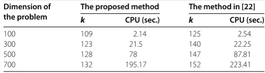
Table 2 Numerical results for problem (5.1) withr= 1,s= 10

Dimension of the problem

The proposed method The method in [22]

k CPU (sec.) k CPU (sec.)

100 109 2.14 125 2.54

300 123 21.5 140 22.25

500 128 78 147 87.81

700 132 195.17 152 223.41

Note that problem (.) is equivalent to the following:

min

X–C

 F+



Y–C

 F

s.t.X–Y= , (.)

X,Y∈Sn₊,

by attaching a Lagrange multiplier Z ∈Rn×n _{to the linear constraintX–Y = , the} Lagrange function of (.) is

L(X,Y,Z) = 

X–C

 F+



Y–C



F–Z,X–Y,

which is defined onSn

+×Sn+×Rn×n. If (X∗,Y∗,Z∗)∈Sn+×Sn+×Rn×nis a KKT point of (.),

then (.) can be converted to the following variational inequality: findu∗= (X∗,Y∗,Z∗)∈

=Sn

+×Sn+×Rn×nsuch that

⎧ ⎪ ⎨ ⎪ ⎩

X–X∗, (X∗–C) –Z∗ ≥,

Y–Y∗, (Y∗–C) +Z∗ ≥, ∀u= (X,Y,Z)∈,

X∗–Y∗= .

(.)

Problem (.) is a special case of (.)-(.) with matrix variables, where A=In×n,B= –In×n,b= ,f(X) =X–C,g(Y) =Y–CandW=Sn+×Sn+×Rn×n.

For simplification, we takeR=rIn×n,S=sIn×nandH=In×nwherer>  ands>  are scalars. In all tests we takeμ= .,C=rand(n) and (X_,Y_,Z_{) = (I}

n×n,In×n, n×n) as the initial point in the test. The iteration is stopped as soon as

maxXk–X˜k,Yk–Y˜k,Zk–Z˜k≤–.

Tables  and  show that the proposed method is more flexible and efficient. Moreover, it demonstrates computationally that the new method is more effective than the method presented in [] in the sense that the new method needs fewer iterations and less com-putational time.

6 Conclusions

In this paper, we propose a new logarithmic-quadratic proximal alternating direction method (LQP-ADM) for solving structured variational inequalities. Each iteration of the new LQP-ADM includes a prediction step, where a prediction point is obtained by using the idea of He [], and a correction step, where the new iterate is generated by a convex combination of the previous iterate and the one generated by a projection-type method along a new descent direction. Global convergence of the proposed method is proved un-der mild assumptions.

Competing interests

The authors declare that they have no competing interests.

Authors’ contributions

All authors read and approved the final manuscript.

Author details

1_{School of Management Science and Engineering, Nanjing University, Nanjing, 210093, P.R. China.}2_{ENSA, Ibn Zohr}

University, BP 1136, Agadir, Morocco.3_{Department of Mathematics, Statistics and Physics, College of Arts and Sciences,} Qatar University, P.O. Box 2713, Doha, Qatar.

Acknowledgements

The authors would like to thank Qatar University for providing excellent research facilities under the Start-Up Grant: QUSG-CAS-DMSP-13/14-8.

Received: 28 April 2014 Accepted: 19 September 2014 Published: 13 October 2014 References

1. Eckstein, J, Bertsekas, DB: On the Douglas-Rachford splitting method and the proximal point algorithm for maximal monotone operators. Math. Program.55, 293-318 (1992)

2. Fortin, M, Glowinski, R: Augmented Lagrangian Methods: Applications to the Solution of Boundary-Valued Problems. North-Holland, Amsterdam (1983)

3. Gabay, D: Applications of the method of multipliers to variational inequalities. In: Fortin, M, Glowinski, R (eds.) Augmented Lagrange Methods: Applications to the Solution of Boundary-Valued Problems, pp. 299-331. North-Holland, Amsterdam (1983)

4. Gabay, D, Mercier, B: A dual algorithm for the solution of nonlinear variational problems via finite element approximations. Comput. Math. Appl.2, 17-40 (1976)

5. Glowinski, R: Numerical Methods for Nonlinear Variational Problems. Springer, New York (1984)

6. Glowinski, R, Le Tallec, P: Augmented Lagrangian and Operator-Splitting Methods in Nonlinear Mechanics. SIAM Studies in Applied Mathematics. SIAM, Philadelphia (1989)

7. Teboulle, M: Convergence of proximal-like algorithms. SIAM J. Optim.7, 1069-1083 (1997)

8. He, BS, Yang, H: Some convergence properties of a method of multipliers for linearly constrained monotone variational inequalities. Oper. Res. Lett.23, 151-161 (1998)

9. Kontogiorgis, S, Meyer, RR: A variable-penalty alternating directions method for convex optimization. Math. Program.

83, 29-53 (1998)

10. Jiang, ZK, Bnouhachem, A: A projection-based prediction-correction method for structured monotone variational inequalities. Appl. Math. Comput.202, 747-759 (2008)

11. Tao, M, Yuan, XM: On theO(1/t) convergence rate of alternating direction method with logarithmic-quadratic proximal regularization. SIAM J. Optim.22(4), 1431-1448 (2012)

12. Chen, G, Teboulle, M: A proximal-based decomposition method for convex minimization problems. Math. Program.

64, 81-101 (1994)

13. Eckstein, J: Some saddle-function splitting methods for convex programming. Optim. Methods Softw.4, 75-83 (1994) 14. He, BS, Liao, LZ, Han, DR, Yang, H: A new inexact alternating directions method for monotone variational inequalities.

Math. Program.92, 103-118 (2002)

15. Hamdi, A, Mishra, SK: Decomposition methods based on augmented Lagrangians: a survey. In: Topics in Nonconvex Optimization: Theory and Applications, pp. 175-204. Springer, Berlin (2011)

16. He, BS: Parallel splitting augmented Lagrangian methods for monotone structured variational inequalities. Comput. Optim. Appl.42, 195-212 (2009)

17. Yuan, XM, Li, M: An LQP-based decomposition method for solving a class of variational inequalities. SIAM J. Optim.

18. Auslender, A, Teboulle, M, Ben-Tiba, S: A logarithmic-quadratic proximal method for variational inequalities. Comput. Optim. Appl.12, 31-40 (1999)

19. Bnouhachem, A, Benazza, H, Khalfaoui, M: An inexact alternating direction method for solving a class of structured variational inequalities. Appl. Math. Comput.219, 7837-7846 (2013)

20. Bnouhachem, A, Xu, MH: An inexact LQP alternating direction method for solving a class of structured variational inequalities. Comput. Math. Appl.67, 671-680 (2014)

21. Bnouhachem, A: On LQP alternating direction method for solving variational. J. Inequal. Appl.2014, 80 (2014) 22. Li, M: A hybrid LQP-based method for structured variational inequalities. Int. J. Comput. Math.89(10), 1412-1425

(2012)

doi:10.1186/1029-242X-2014-392