Combined Compact Difference Scheme for Solving Unsteady Convection Diffusion Equations

(1)

2018 International Conference on Applied Mechanics, Mathematics, Modeling and Simulation (AMMMS 2018) ISBN: 978-1-60595-589-6

Combined Compact Difference Scheme for Solving Unsteady

Convection-Diffusion Equations

Hui BI

*

, Shan LIU, Wei SUN and

Yang SUN

College of Science, Harbin University of Science and Technology, Harbin 150080, China

*Corresponding author

Keywords: Inside point, Boundary, Truncation error, Compact difference scheme, Convection

diffusion equation.

Abstract. By using a fifth-order upwind discrete scheme for the convection term, a fourth-order central difference scheme for the diffusion term, we construct a boundary scheme that matches the interior point and obtain a stable combination semi-discrete compact scheme which is discretized by the third-order Runge-Kutta method in the time direction. Compared with the other fourth-order scheme, the error of the proposed method is small and the accuracy is high.

Introduction

The convection-diffusion equation is widely used in many engineering and practical problems. It is a typical mathematical model for studying the numerical solution of partial differential equations. The usual numerical methods include finite element methods, finite volume methods and finite difference method. Compact difference scheme as a kind of finite difference method is getting more and more attention due to its advantages with fewer grid points and higher accuracy. Hirsh [1] proposed a Hermitian type three-fourth order compact scheme. Lele [2] constructed a class of high accurate compact schemes and gave second, third and fourth order boundary schemes. Tian and Yu [3] derived an unconditionally stable implicit fourth-order accurate difference scheme for one -dimensional unsteady convection-diffusion equations. Wang and Liu [4] used the fourth-order Padé scheme and the four order upwind scheme to discretize the space and time variables respectively and derived a consistent fourth-order compact difference scheme in which the inner point and the boundary are both fourth-order. Zhao [5] used the idea of average weighting to obtain a combined upwind compact scheme with space accuracy at least fourth order. The upwind compact scheme of aerodynamic calculation proposed by Ma and Fu [6] provides an effective method for solving fluid mechanics problems.

In this paper, by using a fifth-order upwind discrete scheme for the convection term, a fourth-order central difference scheme for the diffusion term, we construct a boundary scheme that matches the interior point, and then obtain a stable combination semi-discrete compact scheme which is discretized by the third-order Runge-Kutta method in the time direction. Compared with other fourth-order scheme, the error of the proposed method is small and the accuracy is high.

Scheme Construction

This paper considers the following one-dimensional convection-diffusion equation:

 

     





   

 

 

0

,

 

,



0

,



.

,

0

,

0

,

0

,

0

,

1

u

l

t

g

t

T

g

t

u

l

x

u

T

l

t

x

t

x

f

vu

u

t

x

c

u

_t _x _xx





















₍₁₎

(2)

Spatial Dispersion

We first introduce some notations. Select a positive integerN,M, and lethl/N,





T

/

M

. Write xj 



j1



h_, j1,,N1_{, where}x₁0, xN1l_,tn n _,n0,1,,M_.

n j

u

represents the approximation of the solution functionu

 

x, at pointt



xj,tn



_.

Interior Point Scheme

We use the fourth-order padé scheme [2] to discretize the diffusion term. Let ''

j

u

denote the

approximation of the second-order partial derivative 2

2

x u

 

at pointxj_.

The specific scheme is



1 1



2 ''

1 ''

''

1 2

1 12

1 6 5 12

1

 



  j j  j  j j

j u u u

h u u u

j2,3,,N. (2) The scheme truncation error is

 

6 )

5 ( 4 240

1 _h _u _o_h j 



. (3) The inner point of the convection term is discretized by the fifth-order upwind compact scheme,

where

 

 j x

u

represents the approximation of x

u

 

at point xj_{under the condition of} c0_,

 



j x

u

represents the approximation of x

u

 

at point xj_{under the condition of} c0_.

 



3 44 36 12



3,4, , 1 12

1 3

2 _₁   _  u_₂ u_₁ u  u_₁u_₂ j N h

u

u_x _j _x _j _j _j _j _j _j 

. (4)

 



12 36 44 3



3,4, , 1 12

1 2

3  _₁ _ u _₂ u_₁ u  u _₁ u _₂ j N h

u

u_x _j _x _j _j _j _j _j _j 

. (5) Here we discuss the case ofc0, the truncation error of this scheme is

 6

 

6 5

206

1 _h _u _o_h

j 



. (6) Boundary Scheme

Constructing the diffusion term left boundary scheme [4]



1 1 2 2 3 3 4 4 5 5 6 6 7 7



2 '' 2 1 '' 1

1

u b u b u b u b u b u b u b h u

u        

. (7) The truncation error is

   7

 

6

1 5 7 1

6 1 4 7

1 3

12 19 45

7 180

137 180

13 _b _h _u _b __h _u __o_h

  



 _ _

 

  



 _ _ _ _

. (8) Note this boundary scheme is fourth-order accuracy. In order to keep the boundary and inner point truncation errors (3) consistent [4], we have

   

  

   

1 1

240 1 180

137 180

13

1 7 1



 b

. (9)

Furthermore, we have 720. 597 720

493

7 

(3)

Note that the second item of (8) 7 7 1 13 11 234 11 3 12 19 45 7 b

b  

  

(10) is an increasing function of b7_{. In order to ensure that the truncation error of the boundary scheme}

is closest to the truncation error of the inner point scheme, let 720 494

7 

b

and institute 52 51

1



into(8). Thus, we obtain the following left boundary scheme

          _ _ 

 2 1 2 3 4 5 6 7

'' 2 '' 1 720 494 1040 5063 26 387 936 23914 104 2891 1040 18903 2430 12293 1 52 51 u u u u u u u h u u

. (11) Analogously, we have the right boundary scheme

           _   _ _ _ _ _ _

 2 1 1 2 3 4 5

'' '' 1 720 596 1040 6117 104 1871 936 28735 26 795 1040 17237 4680 17599 1 52 51 N N N N N N N N

N u u u u u u u

h u u

. (12) Combining the interior point scheme (2) with the boundary schemes (11) and (12), we write them

into a matrix form of

U B h U

B 2 2

'' 1 1  , where                                   1 52 51 0 0 0 0 12 1 6 5 12 1 0 0 0 0 12 1 6 5 0 0 0 0 0 0 6 5 12 1 0 0 0 0 12 1 6 5 12 1 0 0 0 0 52 51 1 1        B                            

1 1

3 2 1 2 0 0 0 1 2 1 0 0 0 0 1 2 0 0 0 0 0 0 2 1 0 0 0 0 1 2 1 0 0 0 N N

N b b

b b b b B        1 '' 1 '' '' 1 '' 3 '' 2 '' 1 ''                         N N N N u u u u u u

U  ,

where B1,B2_{are two matrix of}



N1

 

 N1



_{, and}

        U B h B

U'' ₁1 1₂ ₂

.

Next, the boundary scheme of the convection term is constructed. Since the discretize scheme of convection term is a five-point scheme, which fails to calculate the points adjacent to the left and right boundaries which are called the near-boundary points. Therefore, we choose a three-point four-order difference scheme [7] to deal with these near-boundary points.



u u



j N

h u u

u_j''_₁4 _j'' _j''_₁1 3 _j_₁3 _j_₁ 2,

(13)

The truncation error is

 

6 ) 5 ( 4 120

1 _h _u _o_h j 



.

Next, construct the convection term boundary scheme as follows.



1 1 2 2 3 3 4 4 5 5 6 6 7 7



' 2 1 ' 1

1 _a_u _a_u _a_u _a_u _a_u _a_u _a_u

h u

u 



      

. (14) The truncation error is as follow

 6

 

6 1 5 7 1 1237 145 751 2620 4948

57 _a __h _u __o_h

  



 _ _ _

(4)

Same as the calculation method of the diffusion term boundary scheme, we obtain the following left boundary scheme and the right boundary as follows.

         _ _ _ 

 ' ₁ ₂ ₃ ₄ ₅ ₆ ₇

2 ' 1 13907 401 1805 284 931 255 4075 99 1597 806 199 469 597 1207 1 597 0 1 6 u u u u u u u h u

u . (16)

         _ _ _   _ _ _ _ _ _

 1 1 2 3 4 5

' ' 1 1170 229 5986 211 2084 755 29578 427 1463 1954 695 833 1831 145 1 1831 1686 N N N N N N N N

N u u u u u u u

h u

u . (17)

Write the inner point scheme (4) and the boundary schemes (13), (16) and (17) in a matrix form

as:AU h A2U

' 1 1  .                               1 0 0 0 0 0 0 1 4 1 0 0 0 0 0 0 0 3 2 0 0 0 0 0 0 0 3 0 0 0 0 0 0 0 0 0 0 0 0 0 0 0 0 3 2 0 0 0 0 0 0 0 3 2 0 0 0 0 0 0 1 4 1 0 0 0 0 0 0 1 1831 1686 597 610 1          A                                         

 N N

N b b

b b b b b b A 1 2 5 4 3 2 1 2 3 0 3 12 1 12 12 12 36 0 12 1 12 12 12 12 12 36 12 44 12 3 0 12 1 12 12 12 36 12 44 12 3 0 0 3 0 3 0 0 0          1 ' 1 ' ' 1 ' 3 ' 2 ' 1 '                         N N N N u u u u u u U 

where A1,A2_{are two matrixes of}



N1

 

 N1



_.

Furthermore, we have . 1 2 1 1 ' U A A h

U  

Then the semi-discrete equation of the compact difference scheme of the equation (1)is

 

1 12 2 .

1 1 2 1

1 B U

h vB A A h c U

R _    _ (18)

Stability Analysis

According to the stability theory of ordinary differential equations [9], for the semi-discrete equation (18), when the real parts of all eigenvalues of the matrix are negative, the semi-discrete scheme corresponding to the equation is asymptotically stable. Otherwise it is gradual nearly unstable.

Solve the eigenvalues of the matrix 

   _ _    2 1 1 2 1 1

1 B B

h D A A Y

, where c

v D

and the eigenvalues of matrix Y1_{are denoted as}_.

Through the numerical experiments, we found that the scheme is stable whenhis 1/20,1/30,_ 1/100. For example, Figures 1 and 2 show that whenDis taken as 0.01, 0.001, 00010. , respectively and take h as 1/40 and 1/80, the real parts of all eigenvalues of matrix Y1_{are negative. Thus, the}

(5)

Figure 1. h1/40. Figure 2. h1/80.

Numerical Illustrations

Think of the equation as an ordinary differential equation, then

 

u vu'' cu' f .

R dt

du _ _ _ _

For time discretization, we use TVD type third-order Runge-Kutta method [10]

 



 



 





 



 





, 0.5



.

3 2 3 1

, ,

4 1 4 3

, ,

2 2

1

1 1

2 1

t t

u tR u

u u

t t u tR u

u u

t u tR u

u

n n

n n n

  

 



  

 

   



Maximum absolute error L error uiexactuicomput



max

.

To verify the accuracy and reliability of the proposed scheme, consider the constant coefficient convection-diffusion equation with source term:

 

x t f x

u x

u t

u

, 01

. 0 1 .

0 ₂

2

        

,

where f

 

x,t 1.1cos



xt



0.01sin



xt



x

   

0,1,t 0,T .

The exact solution is u

 

x,t sin



xt



, and the initial value is given by the exact solution. The followings are the curves of the numerical solution of the scheme and the exact solution of the equation when the step length changes.

Figure 3. h1/20,T 40. Figure 4. h1/50,T40. Figure 5. h1/100,T40.

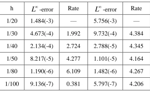
Table 1. Calculation error and convergence order of different grid numbers (t 0.001,T 40).

th

(6)

h _L-error Rate _L-error Rate

1/20 1.484(-3) — 5.756(-3) —

1/30 4.673(-4) 1.992 9.732(-4) 4.384

1/40 2.134(-4) 2.724 2.788(-5) 4.345

1/50 8.217(-5) 4.277 1.101(-5) 4.164

1/80 1.190(-6) 6.109 1.482(-6) 4.267

[image:6.595.176.420.68.215.2]

1/100 9.136(-7) 0.381 5.797(-7) 4.206

Table 1 shows that the error and convergence order of the two schemes under the different step size whenT 40,t0.001, which indicates that the scheme of this paper achieves fourth-order accuracy in space.

Conclusions

Based on the idea of Taylor expansion, this paper constructs a stable boundary scheme with the interior point scheme through the method of undetermined coefficients. Numerical experiments show that the scheme is stability and has fourth-order accuracy.

Acknowledgement

This research was financially supported by the National Natural Science Foundation of China (No. 51406044).

References

[1] R. S. Hirsh. Higher order accurate difference solutions of fluid mechanics problems by a compact differencing technique [J]. Computs. Phys., 1975, (19): 90-109.

[2] S. K. Lele. Compact finite difference schemes with spectral-like resolution [J]. Computs. Phys., 1992, 103(1): 16-42.

[3] Z. F. Tian, P. X. Yu. A high-order exponential scheme for solving 1D unsteady convection difffusion equation [J]. Journal of Computational and Applied Mathematics, 2011(235): 2477-2491. [4] T. Wang, T. G. Liu. A consistent fourth-order compact scheme for solving convection-diffusion equation [J]. Mathematica Numerica Sinica, 2012(4):391-404.

[5] B. X. Zhao. A high-order combined compact upwind difference scheme for solving 1d unsteady convection-diffusion equation [J]. Journal on Numerical Methods and Computer Applications, 2012(2):138-148.

[6] Y. W. Ma, D. X. Fu. A compact scheme and an upwind compact scheme for solving aerodynamic equations[J]. Mathematica Numerica Sinica, 1992(2): 216-223.

[7] C. H. Wang. A class of high-order compact difference scheme for a convection-diffusion equation [J]. Journal of hydrodynamics, 2004, 19(5): 655-663.

[8] F. Tian. A High-Order Compact Exponential-type Finite Difference Scheme on Non-Uniform Grid for Convection-Diffusion Equation [J]. Mathematics in Practice and Theory, 2015(4): 268-275. [9] H. X. Zhang, F. J. Li, Mixed High-order Compact Difference Scheme for Solving the Convection Diffusion Reaction Equation [J]. Mathematics in Practice and Theory, 2017(7): 266-271.