A note on expectational stability under non zero trend inflation

Munich Personal RePEc Archive

A note on expectational stability under

non-zero trend inflation

Kobayashi, Teruyoshi and Muto, Ichiro

28 May 2010

Online at

https://mpra.ub.uni-muenchen.de/22952/

A note on expectational stability under non-zero trend

inflation

Teruyoshi Kobayashi

Ichiro Muto

May 2010

Abstract

This study examines the expectational stability of the rational expectations equi-libria (REE) under alternative Taylor rules when trend inflation is non-zero. We find that when trend inflation is high, the REE is likely to be expectationally unstable. This result holds true regardless of the nature of the data (such as contemporaneous data, forecast, and lagged data) introduced in the Taylor rule. Our results suggest that a high macroeconomic volatility during the period of high trend inflation can be well explained by introducing the concept of expectational stability.

JEL Classification: D84, E31, E52

Keywords: Adaptive learning, E-stability, Taylor rule, trend inflation

∗_{The views expressed here are those of the authors and do not necessarily reflect the official views of the}

Bank of Japan.

†_{Corresponding author. Department of Economics, Chukyo University, 101-2 Yagoto-honmachi,}

Showa-ku, Nagoya 466-8666, Japan. E-mail: [email protected]. Tel, fax: +81-52-835-7943.

‡_{Bank of Japan, 2-1-1 Hongokucho Nihonbashi Tokyo, 103-8660, Japan.}

1

Introduction

Many of the monetary policy analyses based on the New Keynesian framework have ne-glected the existence of non-zero trend inflation. However, several recent studies point out that the introduction of non-zero trend inflation has profound implications for monetary policy. Among them, Kiley (2007) and Ascari and Ropele (2009) introduce alternative versions of Taylor rules into New Keynesian models with non-zero trend inflation. They show that the so-called Taylor principle, which requires the central bank to adjust the nominal interest rate more than one-for-one with the variations of the inflation rate, does not necessarily guarantee the determinacy of the rational expectation equilibrium (REE) when the level of trend inflation is positive. Coibion and Gorodnichenko (2010) recently argue that high trend inflation in the 1970s made the U.S. economy indeterminate even though the Fed’s policy likely satisfied the Taylor principle during that period. This implies that the central bank should carefully choose its policy rule coefficients by recognizing the relationship between the level of trend inflation and the determinacy of REE.

However, these studies assume that the economic agents have perfect knowledge of macroeconomic structures and always form rational expectations. If we instead assume that the agents only have imperfect knowledge and are learning about the structure of the economy over time, then the determinacy of REE is not the sole requirement for the central bank. Bullard and Mitra (2002) propose the expectational stability (E-stability) of REE, which ensures convergence of expectations to the REE under the standard learning algorithm, as another requirement for monetary policy rules. They show the parameter regions that satisfy the E-stability conditions as well as the determinacy conditions under alternative versions of Taylor rules. Their main finding is that the relationship between determinacy and E-stability depends on the version of policy rule being used. However, their study focuses on a relatively specific environment in which trend inflation is exactly equal to zero. It is still unclear how the introduction of non-zero trend inflation will affect their results.

In this study, we attempt to obtain the E-stability (as well as determinacy) conditions of REE, taking into account the presence of non-zero trend inflation. Several previous studies show that the introduction of non-zero trend inflation makes firms’ pricing behavior more

forward-looking compared to the case of zero trend inflation.1

As a result, the rate of current inflation is inevitably affected by long-horizon inflation forecasts. This is the only, but important, departure from the study of Bullard and Mitra (2002).

Our analysis finds that when the level of trend inflation is high, the REE is likely to be E-unstable. This result holds true regardless of the nature of the data (such as contemporaneous data, forecast, and lagged data) used in the Taylor rule. We also show

1_{See, for example, Ascari (2004), Ascari and Ropele (2007), Sbordone (2007) and Cogley and Sbordone}

that while the availability of current economic data in the conduct of monetary policy is a key to E-stability as well as REE determinacy in a low inflation environment, this is not necesarily the case in a high inflation environment.

Our results on E-stability conditions appear to be parallel with Ascari and Ropele’s (2009) finding on determinacy conditions. However, there is an important difference be-tween the two cases. Ascari and Ropele (2009) show that in the case of the lagged-data rule, a rise in trend inflation does not necessarily narrow the determinacy region because the central bank can easily attain determinacy by responding strongly to the lagged out-put gap. In contrast, our study finds that higher trend inflation under the lagged rule makes the REE more likely to be E-unstable even if it is determinate. This means that high trend inflation is more robustly undesirable in terms of E-stability than determinacy. Therefore, the introduction of a learning mechanism can provide a better explanation for the well-established positive relationship between high trend inflation and macroeconomic instability.

2

The model

2.1 A New Keynesian model under non-zero trend inflation

Some previous studies, such as Kiley (2007), Sbordone (2007), Cogley and Sbordone (2008) and Ascari and Ropele (2007, 2009), provide alternative expressions of New Keynesian models under non-zero trend inflation. Our model is based on that of Sbordone (2007) and of Cogley and Sbordone (2008), which is given as follows:

yt = yte+1−σ(it−πet+1−r

n

t), (1)

πt = κyt+b1πe_t+1+b2

∞

j=2

φj1−1π

e

t+j, (2)

rn_t = ρrrtn−1+εt. (3)

πt is the percentage deviation of inflation from the (possibly non-zero) rate of trend

in-flation, which is assumed to be constant. yt, it and rnt are the output gap, the nominal

interest rate and the natural rate of real interest, respectively.2 _{For an arbitrary variable}

x,xedenotes the expectations of variablex. The original AS equation used by Cogley and

Sbordone (2008, eq.8) also includes two additional terms: one is the term that depends on long-horizon forecasts of the output gap, and the other on past inflation. We employ a

2_{Preston (2005, 2006) argues that if adaptive learning is introduced for the process of agents’ expectation}

simpler AS equation because Cogley and Sbordone (2008) show that the estimated

coef-ficients on the additional terms are virtually zero.3

Given the irrelevancy of those terms, our model is essentially the same as the one used by Ascari and Ropele (2007, 2009).

Since firms take into account the influence of trend inflation on their future relative prices, they are more forward-looking under non-zero trend inflation than under zero trend inflation. As a result, long-horizon forecasts emerge in the third term of (2), and thus the

parametersκ,b1,b2 and φ1 are affected by the level of trend inflation.4 In this respect our

framework is distinct from the standard one used in the benchmark work by Bullard and Mitra (2002).

To see how non-zero trend inflation influences firms’ forward-lookingness, it would be

useful to check the values of b1 and b2 under alternative levels of trend inflation. Under

our parameterization, (b1, b2) takes the values of (.968,−.009), (.99,0) and (1.033, .017)

for the rate of (annualized) trend inflation -1%, 0%, 2%, respectively.5

Thus, the sum of coefficients on inflation expectations increases with the level of trend inflation. We also

find that b2 >0 for positive trend inflation and b2 <0 for negative trend inflation. This

implies that the “additional forward-lookingness” stemming from the presence of non-zero trend inflation works in the opposite direction depending on whether the trend inflation is positive or negative.

As for monetary policy rules, we introduce some versions of Taylor rules in which the

central bank responds to (i) the contemporaneous data (yt, πt), (ii) the forecast (yet+1,

πe

t+1), and (iii) the lagged data (yt−1,πt−1). The policy rule is generally given as

it=FlXt−1+FcXt+FfXte+1 (4)

where Xt= [ytπt]′,Fi= [FiyFiπ] fori=c, f, l. c, f and l represent the contemporaneous

rule, the forecast-based rule, and the lagged-based rule, respectively.

2.2 Adaptive learning

We assume that agents estimate their perceived law of motions (PLM) by recursive least squares with decreasing gain, which is the most standard algorithm of adaptive learning

3_{Cogley and Sbordone (2008) report that the degree of price indexation is statistically not different from}

zero, and the estimated coefficient on the long-horizon forecasts of the output gap is at most 5×10−3 over

the whole sample period (1960Q1:2003Q4).

4_{Cogley and Sbordone (2008) derive the parameters as follows: φ}

1 = αβΠ

(θ−1)

, φ2 = αβΠ

θ₍₁₊ω₎

,

χ= 1−α_Π(θ−1)

α₍₁₊θω_)Π(θ−1), b1= (1 + (1 +ω)θχ)φ2−(θ−1)χφ1, b2= (θ−1)χ(φ2−φ1), κ=χ(1−φ2), whereα

is the probability of not changing prices, βis the discount factor,θis the elasticity of substitution among different goods,ωis the responsiveness of real marginal cost to output, and Π is the trend inflation in gross term. The parameter values used in our numerical exercises follow those of Cogley and Sbordone (2008):

α=.588,θ= 9.8 andω=.429. β andσare set at .99 and 6.25, respectively.

5_{In examining the relationship between the E-stability and level of trend inflation, we pay attention not}

(Evans and Honkapohja, 2001). In order to simplify the expression, some previous studies modify the AS equation (2) with an auxiliary variable, which is a linear combination of current output, one-period-ahead inflation forecast and the expectation of the next period’s

auxiliary variable.6 _{This treatment is valid under the rational expectations hypothesis,}

where the economic agents know the functional forms and parameters of the structural equations. However, if we assume that the agents do not have complete knowledge of the functional forms and parameters, then the agents cannot use the auxiliary variable for computing inflation expectations. Therefore, we express the AS equation with long-horizon forecasts without introducing an auxiliary variable.

2.2.1 PLM and ALM: the contemporaneous and the forecast-based rules

Under the contemporaneous rule or the forecast-based rule, PLM is given as

Xt=At+Dtrtn, (5)

where Aand D are 2 by 1 vectors of PLM coefficients. It follows that

∞

j=2

φj−1

1 X

e

t+j = (1−φ1)

−1

φ1At+ (1−φ1ρr)−1φ1ρ 2

rDtrnt. (6)

The structural equations can be reformulated as

QXt=W Xte+1+N it+U rtn+M

∞

j=2

φj1−1X

e

t+j, (7)

where

Q =

1 0

−κ 1

, W =

1 σ

0 b1

, N =

−σ 0 , U = σ 0

, M =

0 0

0 b2

.

By inserting (5) and (6) into (7), we can obtain the actual law of motion (ALM):

Xt = (Q−N Fc)−1{[W +N Ff + (1−φ1)

−1

φ1M]At

+[(W +N Ff + (1−φ1ρr)−1φ1ρrM)ρrDt+U]rnt}. (8)

The T-maps from the PLM to the ALM are then given as

T(At) = (Q−N Fc)

−1

[W +N Ff + (1−φ1)

−1

φ1M]At (9)

T(Dt) = (Q−N Fc)

−1

[(W +N Ff+ (1−φ1ρr)

−1

φ1ρrM)ρrDt+U]. (10)

Here, letDTZ( ¯Z) be the Jacobian matrix of the T-map evaluated at the corresponding RE

value ¯Z:

DTZ( ¯Z) =

∂vec(T(Z))

∂vec(Z)′

Z= ¯Z

.

The E-stability of the REE can be attained if and only if all of the eigenvalues of DTA( ¯A)

and DTD( ¯D) have real parts less than one.

2.2.2 PLM and ALM: the lagged-data rule

Under the rule based on lagged data, it is implicitly assumed that the central bank and the private agents do not have current economic data. McCallum (1999) argues that policymakers are practically unable to obtain the data on contemporaneous macroeconomic variables, such as inflation and output, in making their policy decisions. In this situation it is natural to assume that the private agents also do not have information about current

economic data.7

Therefore, we express the PLM under the lagged-data rule as follows:

Xt=At−1+Ct−1Xt−1+Dt−1r_tn−1, (11)

where expectations formed at time tare based on information aboutt−1-dated variables.

C denotes the 2 by 2 matrix of PLM coefficients. It follows that

X_te+1 = (I+Ct−1)At−1+C 2

t−1Xt−1+ (Ct−1+ρrI)Dt−1rtn−1

X_te+2 = (I+Ct−1+C_t2−1)At−1+C_t3−1Xt−1+ [Ct−1(Ct−1+ρrI) +ρ2rI]Dt−1r_tn−1

X_te+3 = (I+Ct−1+C_t2−1+C 3

t−1)At−1+C_t4−1Xt−1

+[C_t2−1(Ct−1+ρrI) +ρ2rCt−1+ρ3_rI]Dt−1rn_t−1

.. .

The infinite summation term in eq. (2) leads to

∞

j=2

φj1−1X

e

t+j = (1−φ1)

−1

φ1[I+Ct−1+ (I−φ1Ct−1)

−1

C_t2−1]At−1

+(I−φ1Ct−1)−1φ1C_t3−1Xt−1

+(I−φ1Ct−1)

−1

φ1[Ct−1(Ct−1+ρrI) + (1−φ1ρr)

−1

ρ2I]Dt−1rn_t−1

= A˜t−1+ ˜Ct−1Xt−1+ ˜Dt−1rn_t−1.

The ALM can then be written as

Xt = Q−1{W(I+Ct−1)At−1+MA˜t−1+ (W C_t2−1+MC˜t−1+N Fl)Xt−1

+[W(Ct−1+ρrI)Dt−1+ρrU+MD˜t−1]r_tn−1+U εt}. (12)

7_{Bullard and Mitra (2002) also assume this type of informational symmetry. If we instead assume that}

The T-maps from the PLM to the ALM are then given as

T(At−1) = Q

−1

[W(I+Ct−1)At−1+MA˜t−1], (13)

T(Ct−1) = Q

−1

(W C_t2−1+MC˜t−1+N Fl), (14)

T(Dt−1) = Q

−1

[W(Ct−1+ρrI)Dt−1+ρrU+MD˜t−1]. (15)

The E-stability conditions are that all of the eigenvalues of DTA( ¯A,C¯), DTC( ¯C) and

DTD( ¯C,D¯) have real parts less than one.

3

The E-stability conditions under non-zero trend inflation

The combinations of the Taylor rule coefficients, Fiπ and Fiy, i = c, f, l, that ensure

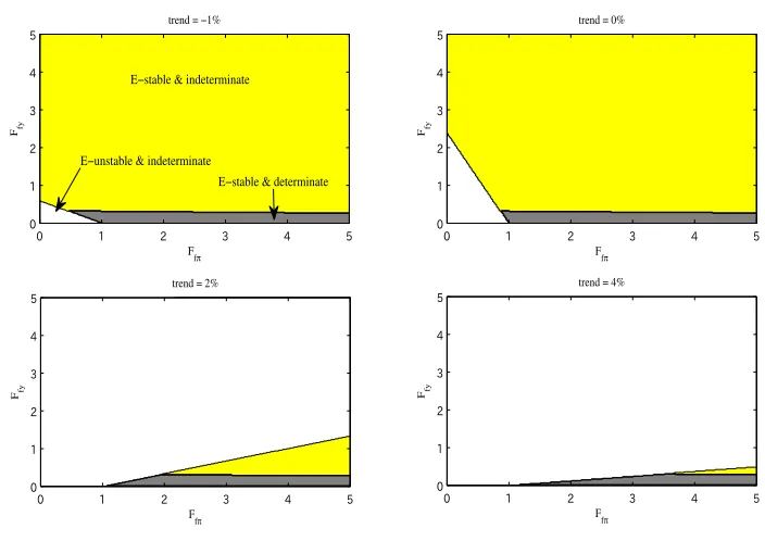
E-stability and determinacy of the REE are presented in Figures 1, 2 and 3. In all figures, the upper-right panel corresponds to the case of zero trend inflation, which is equivalent to the situation analyzed by Bullard and Mitra (2002). The other panels show the E-stable and determinate regions under non-zero trend inflation. Although the determinate regions (except for the case of negative trend inflation) are essentially the same as those presented by Ascari and Ropele (2009), the E-stable regions are novel contribution of our study.

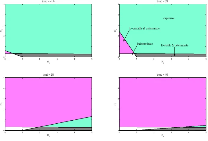
Our main finding is that under all specifications of the rule, higher trend inflation makes REE more likely to be E-unstable: the E-stable region always shrinks as the rate of trend inflation increases. This is in contrast to the case of REE determinacy since higher trend inflation does not necessarily make REE more likely to be indeterminate. Under the contemporaneous rule the E-stable region corresponds exactly to the determinate region, while the E-stable region is broader than the determinate region under the forecast-based rule. In the cases of these two rules, both the determinate region and E-stable region shrink as the rate of trend inflation increases. However, under the lagged-data rule, things are different. In this case, there exists a region in which REE is determinate but E-unstable, as shown by Bullard and Mitra (2002). In Figure 3, we find that this region is broader for higher trend inflation. When the level of trend inflation is high, the central bank can easily achieve the determinacy of REE by responding strongly to the output gap, as is reported by Ascari and Ropele (2009). However, our results show that this kind of policy action fails to make the REE E-stable. Therefore, the REE under the lagged-data rule is more likely to be E-unstable even if it is determinate when trend inflation is high.

that would explain the reduction of macroeconomic volatility following a decline in trend inflation.

Next, let us focus on the case of negative trend inflation. Under all versions of Taylor rules, the determinate and E-stable region is broader when trend inflation is negative rather than positive. Therefore, the REE is less likely to be indeterminate or E-unstable in a deflationary environment. This result has an important policy implication for low inflation countries. If trend inflation is very low, the degree of freedom for the central bank to control the nominal interest rate is inevitably small due to the presence of the zero lower bound (ZLB). Fortunately, our result indicates that the REE is more likely to be E-stable and determinate for lower trend inflation, even when the coefficients of the Taylor rule are small. As a result, the necessity of cutting interest rates against downward shocks will to some extent be removed. This will mitigate the fear of ZLB that the central banks have in an era of very low inflation.

Our analysis also shows that the availability of current economic data for the central bank is especially important in a low inflation environment because, when trend inflation is very low, the E-stable region is much broader under the contemporaneous rule than under the lagged-data rule. However, in a high inflation environment, the E-stable regions are similarly narrow under all versions of Taylor rules. This implies that the central bank’s usage of current economic data does not help much to ensure the E-stability of REE. In this sense, higher trend inflation is very likely to be associated with higher macroeconomic volatility.

4

Concluding remarks

Our analysis has shown that higher trend inflation tends to make REE E-unstable under various specifications of the Taylor rule. This result holds true regardless of the nature of the data employed in the Taylor rule. Although the availability of current economic data for the central bank helps to guarantee the expectational stability of REE in a low inflation environment, this is not necessarily the case in a high inflation environment.

Finally, our main results also have an important implication for the recent dispute on whether the level of inflation targets should be set well above zero. Based on the recent experience of the global financial crisis, Blanchard et al. (2010) raised the issue whether the central bank should aim for a higher inflation target, such as 4%, in normal times in order to avoid ZLB. Our results may provide a negative answer to this question. A rise in the level of trend inflation will change the price-setting behavior of firms in a way that a violation of the E-stability condition becomes more likely. To investigate this issue more formally, however, the influence of ZLB should be explicitly taken into account. This issue should be left for future research.

Acknowledgements

We would like to thank Klaus Adam and Vladyslav Sushko for comments and suggestions. Kobayashi acknowledges financial support from KAKENHI 21243027.

References

[1] Ascari, G., 2004, Staggered prices and trend inflation: some nuisances. Review of Eco-nomic Dynamics 7, 642-667.

[2] Ascari, G. and T. Ropele, 2007, Optimal monetary policy under low trend inflation, Journal of Monetary Economics 54, 2568-83.

[3] Ascari, G. and T. Ropele, 2009, Trend inflation, Taylor principle and indeterminacy, Journal of Money, Credit and Banking 41, issue 8, 1557-84.

[4] Blanchard, O., G. Dell’Ariccia and P. Mauro, 2010, Rethinking macroeconomic policy, IMF Staff Position Note, SPN/10/3.

[5] Bullard, J. and K. Mitra, 2002, Learning about monetary policy rules, Journal of Monetary Economics 49, 1105-29.

[6] Cogley, T. and A.M. Sbordone, 2008, Trend inflation, indexation, and inflation persis-tence in the new Keynesian Phillips curve, American Economic Review 98, 2101-26.

[7] Coibion, O. and Y. Gorodnichenko, 2010, Monetary policy, trend inflation and the Great Moderation: An alternative interpretation, American Economic Review, forth-coming.

[8] Evans, G.W. and S. Honkapohja, 2001,Learning and Expectations in Macroeconomics.

[9] Honkapohja, S., 2003, Discussion of Preston, “Learning about monetary policy rules when long-horizon expectations matter,” Federal Reserve Bank of Atlanta Working Paper 2003-19.

[10] Honkapohja, S., K. Mitra and G.W. Evans, 2002, Notes on agents’

be-havioral rules under adaptive learning and recent studies of monetary policy.

http://darkwing.uoregon.edu/∼gevans.

[11] Kiley, M.T., 2007, Is moderate-to-high inflation inherently unstable? International Journal of Central Banking 3, 173-201.

[12] McCallum, B.T., 1999, Issues in the design of monetary policy rules, in J.B. Taylor

and M. Woodford (ed.),Handbook of Macroeconomics vol 1, Part C, 1483-1530.

[13] Preston, B., 2005, Learning about monetary policy rules when long-horizon expecta-tions matter, International Journal of Central Banking 1, 81-126.

[14] Preston, B., 2006, Adoptive learning, forecast-based instrument rules and monetary policy, Journal of Monetary Economics 53, 507-535.

trend = −1%

F_cπ

Fcy

0 1 2 3 4 5

0 1 2 3 4 5

trend = 0%

F_cπ

Fcy

0 1 2 3 4 5

0 1 2 3 4 5

trend = 2%

F_cπ

Fcy

0 1 2 3 4 5

0 1 2 3 4 5

trend = 4%

F_cπ

Fcy

0 1 2 3 4 5

0 1 2 3 4 5

E−unstable & indeterminate E−stable & determinate

Figure 1: The E-stability and determinacy regions under the contemporaneous rule

trend = −1%

F

fπ

Ffy

0 1 2 3 4 5

0 1 2 3 4 5

trend = 0%

F

fπ

Ffy

0 1 2 3 4 5

0 1 2 3 4 5

trend = 2%

F_fπ

Ffy

0 1 2 3 4 5

0 1 2 3 4 5

trend = 4%

F

fπ

Ffy

0 1 2 3 4 5

0 1 2 3 4 5

E−stable & indeterminate

E−stable & determinate E−unstable & indeterminate

trend = −1%

Fl π

Fl

y

0 1 2 3 4 5

0 1 2 3 4

5 trend = 0%

Fl π

Fl

y

0 1 2 3 4 5

0 1 2 3 4 5

trend = 2%

Flπ

Fl

y

0 1 2 3 4 5

0 1 2 3 4 5

trend = 4%

Flπ

Fl

y

0 1 2 3 4 5

0 1 2 3 4 5

E−unstable & determinate

indeterminate _{E−stable & determinate} explosive