Statistical Investigation and Mapping of Monthly Modified Refractivity Gradient over Pakistan at the 700 Hectopascal Level

http://dx.doi.org/10.4236/ojapr.2016.42005

Statistical Investigation and Mapping of

Monthly Modified Refractivity Gradient over

Pakistan at the 700 Hectopascal Level

Muhammad Usman Saleem1,2

1_{Collage of Earth and Environmental Sciences, University of the Punjab, Lahore, Pakistan} 2_{Institute of Geology, University of the Punjab, Lahore, Pakistan}

Received 23 March 2016; accepted 14 June 2016; published 17 June 2016

Copyright © 2016 by author and Scientific Research Publishing Inc.

This work is licensed under the Creative Commons Attribution International License (CC BY).

http://creativecommons.org/licenses/by/4.0/

Abstract

This study is an effort to investigate the spatial-temporal variability of the modified refractivity gradient at the 700 hPa pressure level over Pakistan and its neighbouring regions of Afghanistan, India, Iran and the Arabian Sea using the remote sensing data of the AQUA (AIRX3STM) satellite from 2008 to 2012. Trapping conditions only found in December were spread over Khyber Pakhtunkhwa (Gilgit-Baltistan, Pakistan) with an average value of −182.042 M/Km and showing Leptokurtic distributions. The lowest monthly average value super-refractive conditions existed in the autumn season with a strong monthly correlation (>0.91 M/Km). A very high monthly correlation (0.9 M/Km) was found for the super-refractive conditions over the whole time period. The largest spa-tial and temporal normal conditions appeared in January with the average value for normal con-ditions being 132.72 M/Km (found over Zabul, Afghanistan) with Leptokurtic distributions. Dur-ing May normal conditions were the smallest in spatial extent over Pakistan, India and Afghanis-tan, showing Platykurtic distributions. Sub-refractive conditions mostly prevailed at all times. The probability for extreme sub-refractive conditions was very high in 2008-2012. The highest aver-age sub-refractive conditions appeared in the winter and autumn seasons (spread around Quetta and Kalam, Pakistan). The highest monthly average sub-refractive conditions with a value of 1,265,188 M/Km were found in January and spread around the Sarbaz River Iran. Correlations for the existence of sub-refractive conditions varied from 0.8 M/Km (moderate strong) to 0.4 M/Km during the autumn to winter season. Permanent super-refractive conditions existed over Balu-chistan from February to September.

Keywords

Atmospheric Refraction, Anomalous Propagation, Ducting

1. Introduction

The major cause of anomalous propagation in the atmosphere is nonstandard atmospheric conditions [1]. Ano-malous propagation conditions in the atmosphere result from the change in atmospheric refractivity with height. This change in atmospheric refractivity is also called duct conditions. These duct conditions create the multipath fading for propagating signals, and the properties of these conditions can be investigated with the average gra-dient of the atmospheric refractive index [2] with geometric height (height above the Earth’s surface). There are two components of atmospheric refractivity, i.e. vertical and horizontal components. The vertical component of atmospheric refractivity is more important than its horizontal component, and the variation of this component in the troposphere (lowest 1 km) is rather linear, and above this is exponential with geometric height [3]. The pro-file of the atmospheric refractivity gradient at a height of 1km above the ground surface is important to study trapping, super-refraction, sub-refraction and ducting phenomena [4]. All weather phenomena such as variation in temperature, density, cloud formation and air pressure take place in the lower troposphere, and in Pakistan tropospheric communications cover the frequencies VHF (30 - 300 MHz) and UHF (300 - 3000 MHz) [5]; even the International Telecommunication Union provides statistics regarding the refractivity gradient within 65 m and 100 m of geometric height [3]. The atmospheric refractivity gradient in the lowest troposphere varies from −500 to

1000 N-units/km [6]. Radio sounding and placing weather sensors on television towers were used to obtain at-mospheric parameters related to atat-mospheric refractivity [7], but radio sounding has mostly been used histori-cally to investigate refractivity profiling in the atmosphere [8]. Using remote sensing techniques to study the profile of atmospheric refractivity is a fairly new topic [9]. Instead of radio refractivity, in practice modified re-fractivity (M) is used, which includes the effect of the curvature of the Earth. In standard atmospheric conditions (recommend by I.T.U) water vapours decrease with height more rapidly than temperature. Atmospheric refrac-tion also decreases with geometric height (height above the Earth’s surface) [10], while modified refractivity in-creases with geometric height. This increase in modified refractivity with geometric height gives better clues to finding the ducting regions in the atmosphere than from the refractivity gradient [11]. When the modified refrac-tivity gradient is constant with geometric height, then the Earth becomes effectively flat to the signal [11]. Dur-ing the ductDur-ing conditions, radar holes form, where radar detection ranges either increase or decrease [12][13]. Reference [10] mentioned the variations in the modified refractivity gradient with a type of anomalous propaga-tion occurring (see Table 1 and Figure 1), and these conditions are very important for radar systems, microwave operations, satellite communications systems and even navigation systems [10].

Ducting is not always wanted due to the interference of reflected rays, variations in lobe pattern, background noise and signal degradation [14]-[17]. In weather applications ducting may lead to coverage fades, false echoes, clutter returns in radar communication, range height errors and acoustic sounders [10]. The incident angle of the radio wave to the ducting boundary is another important factor for surface or air-based systems. The steeper this angle with the boundary layer, the smaller the effect of the ducts on radio propagations [18]. In this paper, we have investigated a modified refractivity gradient using satellite sensed data over Pakistan from 2008 to 2012. Previous work on ducting in Pakistan was done only for Karachi city, which was found to be on point-based data

Table 1. Modified refractivity gradient and corresponding phenomena for the electromagnetic signal propagation.

Conditions Modified Refractivity Gradient (d d M

Z Units) Results (Phenomena Will Occur)

Trapping <0 Trapped: Propagation within the duct boundaries

Super-refraction 0 - 79 Refract downwards towards the Earth’s surface, but at a rate less than the Earth’s curvature but greater than standard

Standard/normal 79 - 157 Refract downwards towards the Earth’s surface with a curvature less than the Earth’s radius

observations or to have a short temporal duration gathered from the Pakistan Naval Authority, the National In-stitute of Oceanography or through radio sounding. This study is the first to investigate a modified refractivity gradient using remote sensing data over Pakistan. We have mapped the modified refractivity gradient by aver-aging the years 2008 to 2012. We have investigated all the propagation conditions occurring over the 700 hec-topascal pressure level. Statistical analysis has been done to investigate propagation conditions over Pakistan and its neighbouring regions of India, Afghanistan, Iran and the Arabian Sea. With the help of these maps and statistical graphs, modified refractivity gradient variations have been investigated seasonally and yearly.

2. Study Area

Pakistan (60˚E - 78˚E, 20˚N - 38˚N) is the 4th

most populated country in Asia. Geographically, China lies to the northeast, Afghanistan to the west, Iran to the southwest, the Arabian Sea to the south and India to the east (see Figure 2). The country has a population of 170.6 million as per 2010 estimates, with a geographical area of

Figure 1. Different cases of the modified refractivity gradient with geometric height.

796,095 km2. One of the major problems in Pakistan is that the changing climate is also changing the environ-ment, temperature and seasons. Its climate varies from arctic-like conditions on snow-covered mountains to ar-id-like conditions in hot desert areas. Southern coastal (including the Arabian Sea) areas have mostly high hu-midity conditions. Taking the whole country’s perspective, the climate is dry. The average annual rainfall varies from area to area, but it has an overall value of about 10 inches annually. The south-western desert area gets less than 5 inches of rain annually, while the eastern Punjab gets more than 20 inches annually. The southern valleys of the Himalayas receive about 70 inches of rain annually. The average coldest temperature for the northern mountainous areas in summer is 23.88˚C. On the Baluchistan Plateau the average temperature is about 26.66˚C in the summer and less than 4.44˚C in the winter.

On the Indus Plain, temperatures range from a high of 32.22˚C to 48.88˚C in the summer, to a low of 12.77˚C in the winter. In the desert regions, temperatures in the hottest months of May and June can reach 50˚C, and the average coldest temperature reaches 5˚C in January. The southern coastal regions have mild, humid weather during most of the year, ranging from 18.88˚C to 30˚C in the winter.

3. Data Set Used

To conduct this study, we have used Atmospheric Infrared Sounder (AIRS) monthly mean geophysical products such as relative humidity (%), surface temperature (K), air temperature (K) and geopotential height (m) at the 700 hPa pressure level. AIRS is one of the instruments mounted onboard the AQUA satellite, which was launched on May 4, 2002 by NASA [19]. The AQUA satellite has 2378 bands in thermal infrared (3.7 - 15.4 µm) and 4 bands in the visible range (0.4 - 1.0 µm). With these spectral ranges the accuracy in atmospheric tempera-ture is 1˚C in 1 km thickness and in relative humidity it is 20% in a layer 2 km thick in the troposphere [18]. The surface temperature, lower tropospheric temperature and water vapor content depend on the nature and proper-ties of the land cover, such as whether it is land, ocean or sea [19]. AQUA crosses the equator during an as-cending orbit at 1:30 PM local time (daytime) and during a desas-cending orbit at 1:30 AM local time (night time). Therefore, we can obtain twice daily geophysical parameters, i.e. humidity, surface temperature, air temperature and geopotential height [19]. We use AIRS level 3 version 5 standard monthly products, which are available on the NASA Goddard Earth Science Data and Information Services Center website [19]. Version 5 has the advan-tage of providing geophysical parameters at 24 pressure levels from 1 to 1000 hectopascal [20]. These geophys-ical parameters have been averaged and bind to a 1˚ × 1˚ grid cell with geographgeophys-ical areas ranging from −180˚ to +180˚ longitude and −90˚ to +90˚ latitude [19]. The standard monthly product has some gaps in satellite data

[19], which we have filled with the averaging of neighbouring values around the missing data.

4. Research Method and Methodology

The data we received from AQUA was in the raw form. We get data of relative humidity (%), geopotential height (m), surface temperature (K) and air temperature (K) over study area from 2008 to 2012 at 700 hPa. With the help of programming in Matlab software, we average this yearly (2008-2012) data into single year. Missing values in data are filled with taking average in the neighbor geographic position.

According to [21], the atmospheric refraction index (n) can be calculated as

6

1 10

n= + ×N − (1)

here N is the dimensionless radio refraction [11] which can be expressed as

77.6

4810

dry wet

e

N N N P

T T

 

= + = _ + _

  (2) Equation (2) consists of two parts, which are given by

77.6

dry

P N

T

= × (3)

5 2 3.723 10 wet e N T

= × (4)

AQUA satellite. These equations are valid for frequencies range up to 100 GHz with less than 0.5% error even also valid for the earth orbiting satellites path [21]. Ndry term contributes about 70% to total value of N[4][7]

and it is the function of temperature and pressure. While the Nwet term contributes to 30% variation of N[7] and

it increases with increasing of relative humidity [22]. The relationship between water vapor pressure (e) and rel-ative humidity (H) is given by:

100

s

He

e= (5)

exp s bt e a t c   = _{ } +

  (6) where H is relative humidity (%), t is average surface ambient temperature (˚C) for the period of a month [23], es

is Saturation vapour pressure (hPa) at the temperature t (˚C). The coefficients a, b, c, are already provided by [21]

(see Table 2).

The saturated vapor pressure (es) from Equation (6) will be in kPa [23] so we have to convert this into hPa.

We have used geometric height over geopotential height due to its independent of atmospheric pressure. In radio propagation it is convenient to use modified refractivity [24] and the formula of modified refractivity which contains the effect of earth’s curvature is given by the following equation

6 10 e z M N R − = +

× (7)

where

N is Radio refractivity form Equation (2).

M is Modified refractivity (dimensionless quantity in M-units).

z is Geometric height, which is the height in meters above the earth’s surface [7][10][24].

Re is Radius of the earth (m).

We have used these conversion between geopotential height (Φ) and geometric height (z) Φ Φ e e R z GR =

− (8)

where

0 g G

g

= (Gravity ratio) (9)

where g0 is the standard average acceleration (value is 9.80665 m/s2) due to gravity at the surface of the earth and g is average gravitational acceleration due to gravity at given latitude, Re is the effective radius. Reference [18] gives the ranges of variation of modified refractivity gradient with geometric height and [25] describe the corresponding phenomena to be appear for the radio signal (seeTable 1). In literature we found variations in the defining for the range of modified refractivity with geometric height [7][13][24] but according to [10], when dM/dz < 0 (M/Km units) then propagation of radio signal will be trapped within duct boundary. Super refraction conditions will be occur when dM/dz = 0 - 79 M/km, in this condition the radio signal will be refracted down-ward to the earth. Normal or Standard conditions occurred when this gradient lies 79 - 157 M/km. Sub refraction condition arises when this value lies above 157 M/km. In this condition radio signal bend upward and move away from the earth [10]. There are two basic types of atmospheric ducts i.e. surface and elevated [20].

Table 2. Values of coefficients recommended by I.T.U.

For water

a = 6.1121 hPa

b = 17.502 hPa

c = 240.97˚C

5. Results and Discussion

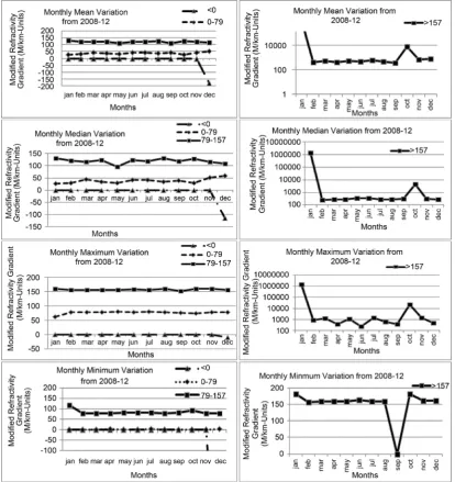
Unfortunately Pakistan lacks the availability of data regarding atmospheric refraction. Only point-based radio sounding observational data are available. We have plotted modified refractivity gradient profiles over the study area. Reference [9] defines duct strength (dM) as the difference in modified refractivity between the top and bottom of the trapping layer. Duct height (dz) is the corresponding geometric height of duct strengths. We find several modified refractivity conditions in a single plot. We have categorized them, and by viewing in the lite-rature [9][21] here we only investigate the first modified refractivity gradient condition occurring in each pro-file. Statistics for each modified refractivity gradient conditions have been calculated and investigated graphi-cally (see Figures 3-5). In each category we have sorted the modified refractivity gradient with values <0, 0 - 79, 79 - 157, >157 M/km. Regions which are not facing these values are replaced with NaN values (missing data), then the statistics of the modified refractivity gradient for each month have been calculated. All the statistical values are given in M/km unit.

Figure 3. Monthly mean, median, minimum values of modified refractivity gradient variation over years (2008-2012). Top left to bottom left column shows these statistical parameters for trapping, super refractive and normal conditions while top

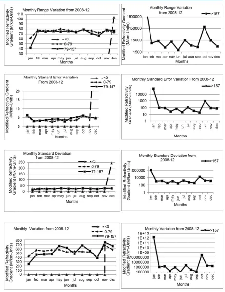
Figure 4. Monthly range, standard error, standard deviations and variance values of modified refractivity gradient variation over years (2008-2012). Top left to bottom left column shows these statistical parameters for trapping, super refractive and normal conditions while top right to bottom right column graphs show corresponding statistical parameters variations for sub

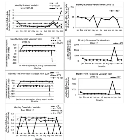
Figure 5. Monthly kurtosis, skewness, 10th percentile and correlation coefficient values of modified refractivity gradient variation averaged over years (2008-2012). Top left to bottom left column shows these statistical parameters for trapping, super refractive and normal conditions while top right to bottom right column graphs show corresponding statistical

parame-ters variations for sub refractive conditions only.

6. Seasonal Statistical Analysis

6.1. Trapping Condition _ _

 

d 0 d

M Z <

December was the only month which shows trapping conditions (d 0 d

M

Z < in M/Km units). Monthly average

(M/Km) lie over Khyber Pakhtunkhwa, Pakistan, with the max value of −10.7751 (M/Km) lying around Thal, Pakistan and the minimum value of −924.582 (M/Km) lying around the Northern Areas of Pakistan (seeFigure 6). The 10th percentile value (the value of trapping conditions below which 10% of the conditions exist) of the trapping condition during this month was −700.098 (M/Km). Trapping conditions of a median value of −115.205

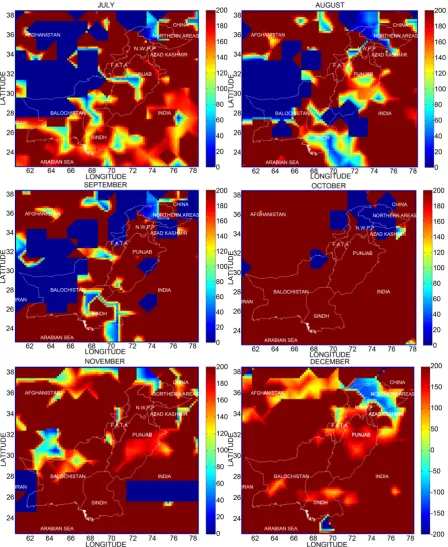
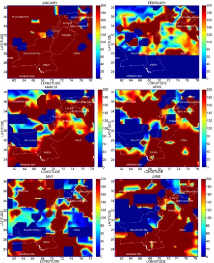
Figure 6. Monthly modified refractivity gradient existence averaged over years (2008-2012) at 700 hPa pressure level. Top

(M/Km) lie near to Gilgit-Baltistan, a Northern Area in Pakistan. Standard deviation describes the variation in trapping conditions around its average value over the study area. The high standard deviation value (245.4459 in M/Km) showed the vast depression in ducting conditions for this month. Variance is the square of standard dev-iation, and its value of 6024.71 (M/Km) again showing a variation of trapping conditions around their monthly average conditions. The kurtosis value (which shows the relative peaks in curves as compared with normal dis-tribution curves) of 4.69648 (M/Km) showed that there were more peaks in the trapping conditions’ distribu-tions than normal distribudistribu-tions, and had flattened tails at the ends. This kurtosis value in December indicated that trapping conditions showed leptokurtic distributions. A skewness of −700.098 (M/Km) showed these dis-tributions are left skewed, and most values of these trapping conditions lie to the right of the mean value of the modified refractivity gradient.

6.2. Super Refraction Conditions _ _

  d 0 79 d M Z < <

This value of the modified refractivity gradient shows the super-refraction conditions which bend the radio sig-nal towards the Earth. The electromagnetic wave moves back towards the Earth with a curvature less than the curvature of the Earth.

6.2.1. Winter Season (December to February)

The average value for the monthly super-refractive conditions varies from 51.167 (M/Km) (lying over Khyar Abad, Afghanistan) to 33.40 (M/Km) (lying over Jammu and Kashmir, India) during December to February. This season has a monthly standard deviation variation from 4.90 (M/Km) to 2.77 (M/Km) in December to Feb-ruary with some high values of 5.68 (M/Km) have been found in January. This means that in December and February the super-refractivity conditions mostly lie near to their average value. Super-refractive conditions oc-curred within the range (the difference of the maximum and minimum super-refractive conditions in a month) of 73.44 M/Km (in December), 62.05 M/Km (in January) and 78.33 M/Km (in February). The kurtosis value in these months was −0.372 (M/Km), −1.241 (M/Km) and −1.030 (M/Km), which indicates that during this season super-refractive distributions have wider peaks than normal distributions. The probability of extreme super-re- fractive conditions during these months was less, and the super-refractive conditions were mostly concentrated around their monthly average values. The skewness value for December (4.03 M/Km), January (1.78 M/Km) and February (1.96 M/Km) indicate that this season has right-skewed distributions with most values of super-re- fractive conditions concentrated on the left of the average super-refractive conditions with extreme values lying to the right of their monthly distributions. The monthly median (middle of the super-refractive conditions) value for super-refractive conditions during these months was 59.35 M/Km (spread over F.A.T.A, Pakistan), 26.601 M/Km (the lowest median value in a year and existing over Kashi, China) and 29.31 M/Km (lying over F.A.T.A, Pakistan), respectively. The monthly mode (most occurrences value) value for super-refractive conditions in December was 71.195 M/Km. The 10th percentile (the value of the modified refractivity gradient below which 10% of the dataset values existed) for super-refractive conditions was 4.039 M/Km (in December), 1.783 M/Km (in January) and 1.956 M/Km (in February). A strong correlation was found between the existences of monthly super-refractive conditions during this season. This correlation value was in December-January (0.88 M/Km), and January-February (0.99 M/Km), indicating that the super-refractive conditions during this season are related closely together. Spatial-temporal variations in super refractive condition in a month will change the super re-fractive conditions of other months for this season.

6.2.2. Spring Season (March to May)

for these months was 43.88 M/Km (in March and found over Lorali, Baluchistan, Pakistan), 33.07 M/Km (in April and lying over Hisor, Tajikistan) and 28.919 M/Km (in May and lying around Haryana, India), respec-tively. The 10th percentile values for super-refractive conditions were 8.76 (M/Km), 10.10 (M/Km) and 4.87 (M/Km), respectively. We have found a strong correlation between monthly super-refractive conditions during this season. The values of this correlation were 0.98 (M/Km), 0.99 (M/Km) and 0.98 (M/Km) during these months in this season.

6.2.3. Summer Season (June to September)

The monthly average value for super-refractive conditions during this season was 39.62 (M/Km) in June (lying over Gilgit-Baltistan, Pakistan), 41.59 (M/Km) in July (lying around Kashmal Gilgit-Baltistan, Pakistan), 36.65 (M/Km) in August (lying around Rajasthan, India) and 39.65 (M/Km) in September (lying over Zhob Baluchis-tan, Pakistan). The standard deviation values for super-refractive conditions were 22.89 M/Km (in June), 23.19 M/Km (in July), 23.01 M/Km (in August) and 22.89 M/Km (in September), showing a strong depression in the occurrence of monthly super-refractive conditions. The monthly range for super-refractive conditions varied from 75 (M/Km) to 78 (M/Km). The monthly median values for these months were 41.88 (M/Km) in June (ly-ing around Fateh Jang, Pakistan), 42.51 (M/Km) in July (ly(ly-ing over Ghor, Afghanistan), 34.15 (M/Km) in Au-gust (lying over the Surukwat Valley in China) and 39.67 (M/Km) in September (lying over Palasava, Rajasthan, India). The monthly kurtosis value remains <3 (M/Km) during this season, showing platykurtic distributions. The skewness (which was >0 M/Km) indicated that during this season the monthly super-refractive distributions were right skewed. Most values of the modified refractivity gradient producing the super-refractive conditions were concentrated on the left-hand side of the average values. The 10th percentile of the modified refractivity gradient during these months was 6.65 M/Km (in June), 8.74 M/Km (in July), 7.49 M/Km (in August) and 3.4389 M/Km (in September). A very strong correlation approximately 0.9 (M/Km) was found in the monthly super-refractive conditions during this season.

6.2.4. Autumn Season (October to November)

The statistics for this season were very interesting to investigate, especially in the case of the monthly average. The lowest average value for super-refractive conditions existed in October (27.06 M/Km and spread around Madhya Pradesh, India) and the second lowest average value for super-refractive conditions (after 51.167 M/Km in December) existed in November (43.07 M/Km and lying over the Shaksgam Valley, Gilgit Baltistan, Pakis-tan). This means that super-refractive conditions during this season were not very strong (seeFigure 6). The standard deviation of values 22.89 M/Km (in October) and 20.344 M/Km (in November) show a low spread of these super-refractive conditions around their monthly average super-refractive conditions. The maximum val-ues of super-refractive conditions for this season were 74.086 (M/Km) in October (found over Farah, Afghanis-tan) and 78.90 (M/Km) in November (spread around the Shaksgam Valley, Gilgit Baltistan, PakisAfghanis-tan). The monthly kurtosis values for super-refractive conditions were 0.899 M/Km (in October) and −1.423 M/Km (in November), suggesting to us that during this season the super-refractive conditions follow the same distributions for means and mode as the super-refractive conditions were facing during the winter. The monthly skewness value suggests to us that right-skewed distributions occurred during this season. The values of the 10th percentile during these months were 1.94 (M/Km) and 5.88 (M/Km), respectively. We have found strong correlations be-tween the October-November super-refractive conditions.

6.3. Normal/Standard Condition _ _

  d 79 157 d M Z < <

This value of the modified refractivity gradient is considered to be standard or normal conditions for radio wave propagations through the atmosphere.

6.3.1. Winter Season (December to February)

Zabul, Afghanistan) and a minimum value for normal conditions of 117.52 M/Km (spread around Karoh, Afg-hanistan). Normal conditions during this season existed within the range of 76.88 (M/Km), 42.26 (M/Km) and 76.25 (M/Km), respectively. The monthly kurtosis <3 (M/Km) and skewness >0 (M/Km) indicate that normal conditions during this season follow leptokurtic distributions in which most values of normal conditions were concentrated to the left-hand side of its monthly average normal values. The probability of the extreme normal

Figure 7. Monthly modified refractivity gradient existence averaged over years (2008-2012) at 700 hPa pressure level. Top

conditions during this season was high. The 10th percentile values for normal conditions during these months were 82.42 M/Km (in December) and 87.98 M/Km (in February). There was no strong correlation for standard conditions during this season.

6.3.2. Spring Season (March to May)

The monthly average values for standard conditions during this season were 118.78 M/Km (in March and exist-ing around Murree, Pakistan), 121.37 M/Km (in April and spread around Tunsa, Punjab, Pakistan) and 110.54 M/Km (in May and found over Heart, Afghanistan). The average normal conditions in May were the lowest compared to the remaining months of the year (see Figure 7). The maximum and minimum values for normal conditions during this month were 155.97 M/Km (spread around Madhya Pradesh, India) and 80.33 M/Km (spread around Surkhandarya, Uzbekistan), respectively. The monthly standard deviation value varies from 21.62 M/Km (in March) to 25.71 M/Km (in May). The kurtosis values in March (−1.00 M/Km), April (−1.07 M/Km) and May (−1.27 M/Km) suggest to us standard conditions follow platykurtic distributions. The skewness for these months were 93.033 M/Km (in March), 90.32 M/Km (in April) and 83.029 M/Km (in May), indicating that most values of standard conditions are concentrated on the left of the monthly average value. The monthly range for normal conditions varies from 75.1 M/Km (in March), 76.19 M/Km (in April) and 75.34 M/Km (in May). The 10th percentile values were 93.033 M/Km (in May), 90.32 M/Km (in April) and 83.029 M/Km (in May). A strong correlation was found only between March-April normal conditions. The remaining months have no correlation for the occurrence of normal conditions.

6.3.3. Summer Season (June to September)

The monthly average values for normal conditions during these months increased in June (122.79 M/Km and existing around Peshawar, Pakistan), July (122.28 M/Km and found over Ahmadwal Railway Station in Balu-chistan, Pakistan) and August (125.75 M/km was the second highest average value for normal conditions and was spread around Yarkand, China), then decreased in September (112.92 M/Km is the second most minimum average value for normal conditions and was found over Takhar, Afghanistan). The standard deviation values during these months were 24.96 M/Km (in June), 21.97 M/Km (in July), 25.99 M/Km (in August) and 23.47 M/Km (in September). The monthly range values for normal conditions during these months were June (76.22 M/Km), July (74.00 M/Km), August (79.4 M/Km) and September (71.03 M/Km). The monthly median values for normal conditions during this season were June 123.93 M/Km (lying around Peshawar, Pakistan), July 118.97 M/Km (lying around Sarbaz River, Iran), August (130.28 M/Km and lying around Punjab, India) and September (117.48 M/Km and lying around Zabul, Afghanistan). During this season normal conditions have 10th percentile values of 90.36 M/Km (in June), 90.90 M/Km (in July), 88.83 M/Km (in August) and 85.61 M/Km (in September). A strong correlation (0.9 M/Km) has been found among June to August normal conditions.

6.3.4. Autumn Season (October to November)

The average value for normal conditions during this season was 126.94 M/Km (in October and it was the second highest average value for normal conditions in a year found around Madhya Pradesh, India) and 120.53 M/Km (in November and existing around the Punjab, India). The monthly median values for normal conditions during these months were 128.98 M/Km (the second highest value for normal conditions and found over Madhya Pra-desh, India) and 115.16 M/Km (the second lowest value for normal conditions and found over Uttarakhand, In-dia). Normal conditions vary in range values of 67.047 M/Km (in October) to 78.93 M/Km (in November). The kurtosis value <3 M/Km during these months suggest this season was facing platykurtic distributions. The monthly skewness values during these months were 93.60 M/Km (in October) and 82.27 M/Km (in November), which is >0 M/Km, indicating that normal conditions followed right-skewed distributions. The value of the 10th percentile for November was 82.27 M/Km and there existed a strong correlation value of 0.959 M/Km between November-December normal conditions.

6.4. Sub Refraction Condition _ _

  d 157 d M Z >

Sub-refraction conditions prevail with this d 157 M Km

(

)

M

the modified refractivity gradient value becomes >157 M/Km then the electromagnetic signal will bend upwards, away from the Earth’s surface.

6.4.1. Winter Season (December to February)

The sub-refractive conditions during the winter season were interesting to investigate (seeFigure 6 and Figure 7). The mean values for the modified refractive gradient during these months were 768.58 M/Km in December (lying around Kalam, Pakistan), 1,265,188 M/Km in January (the highest value in the year and spread around the Sarbaz River, Iran) and 445.14 M/Km in February (lying over Ghazi, Afghanistan). In January the monthly average sub-refractive conditions were found to be maximum, and we have found the reason to be due to the very high amount of duct strength during this month (see Figure 7). The standard deviations for these months were 1294.159 M/Km (in December), 1,190,731 M/Km (in January) and 1001.68 M/Km (in February). These high values of standard deviation in the month of January indicate high variations of sub-refractive conditions around its average value over the study area. The monthly maximum value for sub-refractive conditions is 4811.667 M/Km (in December and existing over Godhra, India), 14,042,367 M/Km (January and spread around Gwalior, India) and 9315.469 M/Km (for February and existing over Heart, Afghanistan). The monthly ranges for sub-refraction were in December (4649.398 M/Km), January (14,042,184 M/Km) and February (9315.469 M/Km), respectively. The kurtosis value >3 M/Km showed that monthly sub-refractive conditions follow lepto-kurtic distributions in which most sub-refractive conditions were concentrating around their average value, and these distributions have sharper edges with long tails. The probability of extreme monthly values for sub-re- fractive conditions during this season was very high. The monthly skewness values >0 M/Km tells us that the sub-refractive conditions were right skewed. This means that most monthly sub-refraction conditions concen-trated to the left of their monthly average values. This season has monthly median values of 280.88 M/Km (for December), 1,405,304 M/Km (for January) and 239.4459 M/Km (for February). The monthly mode values for December and January are 172.7128 M/Km and 139,908 M/Km, respectively. The minimum values of sub-re- fraction conditions were 162.269 M/Km (in December and existing over Herat, Afghanistan), 182.47 M/Km (in January and existing over the Shaksgam River, Northern Area in Pakistan) and 170.77 M/Km (in February spread around the Northern Area, Pakistan). The 10th percentile for sub-refractive conditions was for December (191.148 M/Km), January (496.187 M/Km) and February (170.77 M/Km). The monthly correlation for these months was going to increase from weak (0.38 M/Km) to moderately strong (0.804 M/Km) during December to February.

6.4.2. Spring Season (March to May)

The monthly mean values for sub-refractive conditions were 527.252 M/Km (in March and spread around Ra-jasthan, India), 423.50 M/Km (in April and it was the lowest monthly value of sub-refractive conditions in the year which was spread around Bahawalpur, Pakistan) and 546.437 M/Km (in May and existing over Rajasthan, India) (see Figure 6). The most occurring values for sub-refraction were 285.57 M/Km and 216.61 M/Km in March and April, respectively. The median values for sub-refractive conditions during these months were 239.44 M/Km, 291.025 M/Km and 359.083 M/Km, and the monthly kurtosis value >3 M/Km indicates that during this season sub-refractive conditions follow leptokurtic distributions. Skewness values remaining >0 M/Km indicate that these sub-refractions follow right-skewed distributions. The 10th percentile values for these months were 190.97 M/Km (in March), 192.18 M/Km (in April) and 189.063 M/Km (in May). Moderately strong to strong correlations were found for the sub-refractive conditions during this season.

6.4.3. Summer Season (June to September)

remain >3 (M/Km), which indicates that leptokurtic distributions existed for sub-refractive conditions during this season. These distributions were right skewed. The standard deviation varies from 315.57 M/Km (in June), 1527.374 M/Km (in July), 557.7699 M/Km (in August) and 341.655 M/Km (in September). The 10th percentile values for these months were 203.77 M/Km (in June), 171.172 M/Km (in July), 183.97 M/Km (in August) and 51.788 M/Km (in September). The correlation for the sub-refractive conditions were going to change from strong (0.9267 M/Km in June) to moderately strong (0.73 M/Km in July, 0.79 M/Km in August) and again strong (0.804 M/Km in September) (seeFigure 5).

6.4.4. Autumn Season (October to November)

The monthly average sub-refractive conditions vary from 7931 M/Km (in October and lying around Quetta, Pa-kistan) to 697.58 M/Km (in November and lying around Farah, Afghanistan). The median values of 4434.842 M/Km (in October and spread around Gizab, Afghanistan) and 307.50 M/Km (in November and spread around Jodhpur, India) were found for sub-refraction during this season (see Figure 7). The monthly standard devia-tions during these months were 16465 M/Km (in October) and 1462.485 M/Km (in November). The sub-re- fractive conditions vary in range from 216,980 M/Km (in October) to 14,867.9 M/Km (in November). The monthly kurtosis value was >3 M/Km, indicating that in each month sub-refractive conditions follow leptokurtic distributions. The skewness value >0 M/Km indicates that these distributions were right skewed, where most sub-refraction values were concentrated on the left of the average sub-refractive conditions, while extreme sub-refractive conditions existed to the right of the mean sub-refractive conditions. The 10th percentiles for the sub-refractions during these months were 0.77 M/Km (in October) and 197.96 M/Km (in November). During this season there was a moderately strong (0.77 M/Km in October-November) to strong (0.845 M/Km in No-vember-December) correlation existing for the sub-refraction conditions.

7. Yearly Statistical Interpretation

In the literature, mostly univariate or bivariate statistical analysis has been done to investigate anomalous prop-agation [3][4][7][8][10] [11][26][27]. So we have calculated the monthly mean, median, mode, standard deviations, standard error, variance, maximum, minimum, range, kurtosis, skewness, and correlations and made plots of them against each month to investigate the yearly variations of these parameters (see Figures 3-5). In

d

157 M Km d

M

Z > we got very high values for the modified refractivity gradient, which is why we made a plot

of them separately (seeFigures 3-5). Trapping conditions occur only in December. The monthly mean, median, maximum, minimum, range, standard deviation, kurtosis, skewness and 10th percentile values of the modified refractivity gradient follow the same pattern of variability yearly; even some time increment in the modified re-fractivity for three cases of propagation, e.g. super-refractions, normal and sub-refractions follow the same pat-tern of variability throughout the year (seeFigures 3-5). Yearly correlation coefficient variations tell us those super-refractive conditions show a strong correlation throughout the year (see Figure 5). This strong correlation between months remains from the spring to the summer season, but in the autumn and winter seasons these su-per-refractive conditions have moderately strong correlations (around 0.89 M/Km). Normal conditions for radio propagations show very strong correlations (0.9 M/Km) during the spring season (February to April), the sum-mer season (May to September), the autumn season (November to December) with no correlation (0 M/Km) in April-May, September to October, and December to January normal conditions (see Figure 5). The winter sea-son (December to February) shows a moderate correlation (around 0.5 M/Km) for sub-refractive conditions. During the spring season this correlation coefficient varies between strong (0.9 M/Km and found in March-April conditions) to moderately strong (0.8 M/Km and found in February to March, April to May conditions). Whe-reas in the summer season this correlation for the sub-refractive conditions decWhe-reases from strong (0.9 M/Km in the months of May to June) to moderately strong (around 0.8 M/Km in July to September), and this moderate correlation prevails in the autumn season for sub-refractive conditions (see Figure 5).

8. Mapping Modified Refractivity Gradient

8.1. Trapping Condition (Ducting Conditions)

in-vestigate these ducting conditions appearing around the Gulf of Kutch (India), Northern Areas (Gilgit-Baltistan), Azad Kashmir (Pakistan) and Jammu Kashmir (India) with a vast spatial extent.

8.2. Super Refractive Conditions

During the winter season, super-refractive conditions mostly prevailed over the Punjab (Pakistan), N.W.F.P, F.A.T.A, Baluchistan (Killa, Mastung) and the Northern Areas of Pakistan. February was the month when vast spatial extent super-refractive conditions existed over Pakistan (see Figure 7). During the spring season these super-refractive conditions remain persistent over Baluchistan (also on Gwader Port), F.A.T.A, and Northern Areas of Pakistan (see Figure 7). In May super-refractive conditions spread over the Punjab (Lahore, Faisalabad, Gujranwala and Gujarat), and even over the Punjab and Haryana provinces of India. During the summer season Baluchistan, F.A.T.A (Wana Airport), Northern Areas (Pakistan), Iran and Afghanistan (Pakita, Zabul, Khaddar, Helmand, Nimuz and Farah) face super-refractive conditions for electromagnetic wave propagations. The au-tumn season has the smallest spatially super-refractive condition occurrence (see Figure 6). In October much fewer super-refractive conditions appear over Northern Areas (a region in Pakistan) and Azad Kashmir (a region in Pakistan). November was the month in which no super-refractive condition appear over Pakistan (see Figure 6).

8.3. Normal or Standard Conditions

During the winter season normal conditions mostly appeared over the Punjab (Pakistan and India), F.A.T.A and Baluchistan (Ghowal Zhob); even one normal condition appeared over Northern Areas (a region in Pakistan) and Jammu and Kashmir (India) (seeFigure 6 and Figure 7). January was the month in which no normal condi-tions appear over Pakistan (see Figure 7). During the spring season these normal conditions remain persistent over the Punjab (Pakistan), but at the end of the spring season these normal conditions become very weak in ex-tent over Pakistan (see Figure 7). In summer season these normal conditions appear over Sindh, the Arabian Sea and even over the Rajasthan province of India. July and August were the months when vast spatial extent normal conditions appear over Sindh (Pakistan) and the coastal areas of Baluchistan (see Figure 7). In October (autumn season) no normal conditions existed over Pakistan with very few normal conditions appearing over the Punjab (Lahore, Faisalabad, Multan) in November.

8.4. Sub Refractive Conditions

With the start of the winter season sub-refractive conditions spread over the Punjab (Bahawalpur, Dara Ghazi Khan), Baluchistan, Sindh, the Arabian Sea, Afghanistan and India. January was the month in this season when vast spatial extent sub-refractive conditions exist over Pakistan, India, the Arabian Sea and Afghanistan (see Figure 7). During the spring season these conditions remain over Sindh, N.W.F.P and the Punjab (Pakistan). With the start of the summer season these sub-refractive conditions spread over the Punjab (Pakistan and India), Sindh, the coastal areas of Baluchistan and F.A.T.A (see Figure 7). High and low spatial in extent sub-refractive conditions appear in July and August during this season. During the autumn season large spatial in extent sub-refractive conditions appear over Pakistan (see Figure 6). October and November were the months after January in which high sub-refractive conditions appear.

9. Conclusion

December is the only month in which trapping conditions were prevailing. Super refractive conditions were found to have strong correlation in all time. Lowest average normal conditions were found in spring season. There was no correlation in normal conditions of winter and spring seasons. Moderate to strong correlation was found in appearance of sub refractive conditions.

Acknowledgements

References

[1] Uz-Zaman, M. and Zafar, T. (2014) To Investigate the Performance of Microwave Communications in a Strong Me-teorological Ducting Environment in Pakistan Southern Region. Science International, 26, 1423.

[2] Sasaki, O. and Akyama, T. (1982) Studies on Radio Duct Occurrence and Properties. IEEE Transactions on Anntennas and Propagation, 30, 853-858. http://dx.doi.org/10.1109/TAP.1982.1142921

[3] Mufti, N. and Siddle, D. (2013) Investigations into the Initial Refractivity Gradients and Signal Strengths over the Eng-lish Channel. 7th European Conference on Antennas and Propagation, Gothenburg, 8-12 April 2013, 1691-1694.

[4] Willoughby, A., Aro, T. and Owolabi, I. (2002) Seasonal Variations of Radio Refractivity Gradients in Nigeria. Jour-nal of Atmospheric and Solar-Terrestrial Physics, 64, 417-418, 421. http://dx.doi.org/10.1016/s1364-6826(01)00111-0 [5] Waheed-uz-Zaman, M. (2013) To Study the Implications of the Evaporation Duct for Ground Waves Path in Pakistan

Coastal Water through Statistical Assessment. Journal of American Science, 9, 524-527.

[6] Mufti, N. (2011) Investigation into Effects of the Troposphere on Vhf and Uhf Progation and Interference between Co Frequencies Fixed Links. University of Leicester, UK.

[7] Falodun, S. and Sjewole, M. (2006) Radio Refractive Index in the Lowest 100-M Layer of the Troposphere in Akure, South Western Nigeria. Journal of Atmospheric and Solar-Terrestrial Physics, 68, 8236-8242.

http://dx.doi.org/10.1016/j.jastp.2005.10.002

[8] Grabner, M. and Kvicera, V. (2006) Refractive Index Measurements in the Lowest Troposphere in the Czech Republic. Journal of Atmospheric and Solar-Terrestrial Physics, 68, 1334-1339. http://dx.doi.org/10.1016/j.jastp.2006.05.005 [9] Von Engeln, A. and Teixeira, J. (2004) A Ducting Climatology Derived from the European Centre for Medium-Range

Weather Forecasts Global Analysis Fields. Journal of Geophysical Research, 109. http://dx.doi.org/10.1029/2003jd004380

[10] Mentes, S. and Kaymaz, Z. (2006) Investigation of Surface Duct Conditions over Istanbul, Turkey. Journal of Applied Meterology and Climatology, 35, 318-329.

[11] Babin, S. (1995) Surface Duct Height Distributions for Wallops Island, Virginia, 1985-1994. Journal of Applied Mete-orology, 35, 86-87, 89-91. http://dx.doi.org/10.1175/1520-0450(1996)035<0086:SDHDFW>2.0.CO;2

[12] Reddy, K.K., et al. (2010) Lower Atmospheric Wind Profiler at Gadanki, Tropical India: Initial Results. Meteorolo-gische Zeitschrift, 10, 457-468. http://dx.doi.org/10.1127/0941-2948/2001/0010-0457

[13] Douvenot, R., Fabbro, V., Gerstoft, P., Bourlier, C. and Sillard, J. (2008) A Duct Mapping Method Using Least Squares Support Vector Machines. Radio Science, 43, 1-2. http://dx.doi.org/10.1029/2008RS003842

[14] Rana, D., Webster, A.R. and Sylvain, M. (1992) Statistical Characterization of Line-of-Sight Microwave Links. Radio Science, 7, 783-796. http://dx.doi.org/10.1029/92RS01151

[15] Webster, A. (1997) Extended Observations of Fading on a Terrestrial Microwave Link. Radio Science, 32, 231-238. http://dx.doi.org/10.1029/96RS02789

[16] Sukra, J. (1987) Worldwide Anomalous Refraction and Its Effects on Electromagnetic Wave Propagation. John Hopk-ing Digest. http://www.jhuapl.edu/techdigest

[17] Ko, H., Sari, J. and Skura, J. (1983) Anomalous Microwave Propagation through Atmospheric Ducts. John Hopking Technical Digest. http://www.jhuapl.edu/techdigest

[18] Patteron, W., Hattan, C., Lindem, G., Paulus, R., Hitney, H., Anderson, K. and Barrios, A. (1994) Engineer’s Refrac-tive Effects Prediction System. Naval Research and Development Technology.

[19] DES DISC (2008) Readme Document for AIRS Level 3 Version 5 Standard Probuct. NASA.

[20] Saleem, M. (2015) Atmospheric Ducts: Their Application in Radio Frequency Propagation Using Remote Sensing Techniques. Lap Academic Publisher, Saarbrücken.

[21] Recommendation ITU-R (1997) The Radio Refractive Index: Its Formula and Refractivity Data. ITU.

[22] Rao, S.G.V.R.K. and Purnachandra Rao, M., (2007) Addendum to “Study on Coastal Atmospheric Effects on Line of Sight Links Located in Visakhapatnam”. AU Journal of Technology, 10, 276-278.

[23] Ippolito, L. (2008) Satellite Communications Systems Engineering. Weily, Chichester. http://dx.doi.org/10.1002/9780470754443

[24] Rogers, L. (1997) Likelihood Estimation of Tropospheric Duct Parameters from Horizontal Propagation Measurements. Radio Science, 32, 79-80. http://dx.doi.org/10.1029/96RS02904

[25] Hitney, H., Richter, J.H., Pappert, R.A., Anderson, K.D. and Baumgartner, G.B. (1985) Tropospheric Radio Propaga-tion Assessment. Proceedings of the IEEE, 73, 265-283. http://dx.doi.org/10.1109/PROC.1985.13138

in Karachi, Pakistan. 12ThInternational Bhurban Conference on Applied Sciences and Technology, Karachi, 13-17 January 2015, 617-619. http://dx.doi.org/10.1109/ibcast.2015.7058569