Experimental Study on the Cyclic Ampacity and Its
Factor of 10 kV XLPE Cable
Xiaoliang Zhuang, Haiqing Niu, Junfeng Wang, Yong You, Guanghui Sun
School of Electric Power, South China University of Technology, Guangzhou, China Foshan Power Bureau of Guangdong Power Grid Company, Foshan, China
Email: [email protected] Received April, 2013
ABSTRACT
The load varies periodically, but the peak current of power cable is controlled by its continuous ampacity in China, re-sulting in the highest conductor temperature is much lower than 90℃, the permitted long-term working temperature of XLPE. If the cable load is controlled by its cyclic ampacity, the cable transmission capacity could be used sufficiently. To study the 10 kV XLPE cable cyclic ampacity and its factor, a three-core cable cyclic ampacity calculation software is developed and the cyclic ampacity experiments of direct buried cable are undertaken in this paper. Experiments and research shows that the software calculation is correct and the circuit numbers and daily load factor have an important impact on the cyclic ampacity factor. The cyclic ampacity factor of 0.7 daily load factor is 1.20, which means the peak current is the 1.2 times of continuous ampacity. If the continuous ampacity is instead by the cyclic ampacity to control the cable load, the transmission capacity of the cable can be improved greatly without additional investment.
Keywords: XLPE Cable; Experiment; Cyclic Ampacity; Software
1. Introduction
Power cable has been widely used in urban power grids. With the rapid economic development in China, the transmission capacity of power cable needs to be im-proved. However, it is extremely difficult to construct new cables due to the high cost and the dense under-ground pipeline in urban [1]. Therefore, it is very impor-tant to take full advantage of the cable capacity.
In China, the cable load is adjusted based on its rating, i.e. the continuous ampacity. However, the actual current in operation cable is not continuous but showing a peri-odical variation. What’s more, the daily load curve shape doesn’t change a lot within a relatively long period of time (such as one month). Due to the existence of ther-mal capacity of cable system (including the cable and its surrounding soil), the cable conductor temperature (namely insulation temperature) is delayed hours after the load changes, the delay time depend on its thermal time stant. In this situation, if the cable peak current is con-trolled by its continuous ampacity, the highest cable conductor temperature will be much lower than 90℃, which is the permitted long-term working temperature of XLPE, resulting in a waste of the current carrying capac-ity. If using the cyclic ampacity to control the cable load, its transmission capacity can be improved greatly without any additional investment [2].
IEC 60853 standards have given the calculation meth- ods of the cable cyclic ampacity factor and the cyclic ampacity [3,4], with condition that the conductor tem-perature will up to but not exceeding the maximum al-lowable cable insulation working temperature. In order to bring the transmission capacity of 10kV distributed cable lines into full apply, a three-core cable cyclic ampacity calculation software is developed and the cyclic ampacity experiments of direct buried cable are undertaken in this paper, and also the software calculations are used to do theoretical research. There are few articles about the cy-clic in domestic now, but these experiments can provide some experiences and references for future related re-searches.
2. Experimental Study Content
2.1. Test Object and Ground
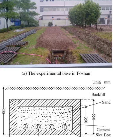
Experiments are undertaken in Foshan experiment field, shown in Figure 1(a). Cables are located in the cement tanks box filled with sand, which is buried in the soil, shown in Figure 1(b). The depth of cable is 700 mm, the length of cable is 20 m and the cable is YJV22-8.7/ 15-3 × 240.
2.2. Selection of Daily Load Curve
and hybrid four typical load, this project select 10 lines to analyze the daily load factor, which is defined as formula (1) [5]. Considering the daily load curves in one month are almost the same, we select a typical load curve, the maximum one, in one month. 33 daily load curves, im-ported from Foshan Power Supply Bureau SCADA sys-tem of 33 months (from January 2009 to Sepsys-tember 2011), are used to calculate the daily load factor.
(a) The experimental base in Foshan
(b) The sectional view of laying of the experimental cables
Figure 1. Schematic diagram of cable laying method.
0 max
1
( )
t
LF I t dt
I
(1)For the load current is adjusted in every 15 minutes, each daily load curve data will have 96 data per day. Discretization of the formula (1) can be rewritten as:
96 1 max
(t)
96
I LF
I
(2)
Typical daily load curves of LF 0.5, 0.7, 0.8, and 0.9 are selected to control the current applied in experiments. The red curve in Figure 2 is the selected load with0.7 daily load factor.
2.3. The Direct Burial Experiment
Single-loop cyclic ampacity experiments of direct buried cable are carried out with the daily load factor 0.5, 0.7, 0.8, 0.9 and 1 (i.e. the continuous load) and four-loop cyclic ampacity experiments with 0.7 daily load factor.
[image:2.595.77.269.194.426.2] [image:2.595.312.534.291.424.2]During the experiment, cyclic current is loaded in the cables according to the selected load curves while re-cording the temperature of the cable conductor and skin by thermocouple. Adjust the peak current every day but keep the load curve shape till the conductor temperature is about 90℃(the highest permitted temperature of XLPE insulation) and get a named quasi static state, which is defined as the difference of the conductor temperature and peak current between the last two days are less than 2℃and 5% respectively. In this situation the peak current of the last cyclic is defined as the cyclic ampacity [6-10].
Figure 2 shows the procedure of current, conductor
temperature, the skin temperature and the surrounding soil temperature in the cyclic ampacity experiment. Ta-ble 1 and Table 2 show the results of cyclic ampacity experiments of the single-loop and four-loop.
0 1000 2000 3000 4000 5000 6000
10 20 30 40 50 60 70 80 90 100
Time/min
T
em
p
er
at
u
re/
℃
0 1000 2000 3000 4000 5000 60000
100 200 300 400 500
Cu
rr
en
t/
A
current
conductor temperature
shealth temperature soil temperature
[image:2.595.307.539.491.594.2]Figure 2. Graph of LF 0.7 single-loop direct buried cable cyclic ampacity experiment.
Table 1. Results of cyclic ampacity experiment of the single- loop cable.
[image:2.595.309.539.633.736.2]LF 0.5 0.7 0.8 0.9 1 Cyclic ampacity /A 528.3 487.9 545.1 531.1 380 Maximum conductor temperature/℃ 92.0 90.7 89.7 89.5 91.1 Maximum skin temperature/℃ 73.7 73.5 72.4 72.4 81.7 Ambient temperature/℃ 18.3 18.3 19.9 18.7 23.1
Table 2. Results of cyclic ampacity experiment of the four- loop cable.
LF 0.7 1
Cyclic ampacity /A 344.0 268.0
3. Comparison of the Experiment and
Calculation
paper, as shown in Table 3 and Table 4 respectively. As comparison, the experiment results are also show in Ta-ble 3 and Table 4.
3.1. The Calculation of Cable Cyclic Ampacity
According to IEC60853 standard, cyclic ampacity is equal to cyclic ampacity factor M multiplied by the con-tinuous ampacity [4].
1
5 ( 1) ( ) (6)
1
( ) ( ) ( )
0
R R R
i
R R R
M
i i
Y i
(3)
It can be seen from Table 3 and Table 4 the maximum error of the calculation and the experiment of the single- loop and four-loop are -3.6% and -0.2% respectively, showing the correctness of the calculation of the cable cyclic ampacity.
3.3. Comparison of the Calculation and Experiment of Cyclic Ampacity Factor M
where: The thermal resistance coefficients of surrounding media and the ambient temperatures are different in ments. To get the cyclic ampacity factor M, the experi-ments are corrected from experiment condition to the standard condition, that is with 1.2 K•m/W thermal re-sistance coefficients of surrounding media and 30℃ ambient temperature.
Yi is the function of cyclic load factor; R( )i is the
temperature rise of i-th hour; R( ) is the steady-state temperature rise of continuous current conductor; μ is the cyclic load-loss factor.
If the cyclic ampacity is used to control the cable load, the highest conductor temperature of cable will reach but not exceed 90℃, which is the allowed long-term working temperature of XLPE. Three-core cable cyclic ampacity calculation software has been developed according to IEC60853 standards.
By the 10kV cable ampacity calculation guide, the experimental are corrected to standard condition, and the results are shown in Table 5 and Table 6. According to the results, calculated values and experimental values are about the same. The experiment value of cyclic ampacity factor is the ratio of experiment result of cyclic ampacity to continuous one. The cyclic ampacity factor could be calculated by the software. Table 5 and Table 6 shows cyclic ampacity factor of experiment and calculation. 3.2. Comparison of the Calculation and the
Experiments of Cyclic Ampacity
The cyclic ampacity experiments of the single-loop and four-loop are calculated by the software developed in this
Table 3. Cyclic ampacity experiments and the calculation of the single-loop cable.
0.5 0.7 0.8 0.9 1 LF
experimental values / calculated values
experimental values / calculated values
experimental values / calculated values
experimental values / calculated values
experimental values / calculated values
Cyclic ampacity /A 528/535 488/487 545/563 531/512 380/371 Error 1.3% -0.2% 3.3% -3.6% -2.4%
Table 4. Cyclic ampacity experiment and calculation of the four-loop cable.
LF0.7 single loop four loops experimental values / calculated values Test values / calculated values Cyclic ampacity /A
488/487 344/343.5
Error -0.2% -0.1%
Table 5. Comparison results of the single-loop direct buried cable cyclic ampacity experiment under the standard condition.
0.5 0.7 0.8 0.9 1 LF
experimental values / calculated values
experimental values / calculated values
experimental values / calculated values
experimental values / calculated values
experimental values / calculated values
Table 6. Comparison results of the four-loop direct buried cable cyclic ampacity experiment under the standard condi-tion.
LF0.7 single loop four loops test values 536 417.4 Cyclic ampacity /A
calculated values 554 405 test values 1.22 1.35 M
calculated values 1.20 1.26
From Table 5, the M with 0.5, 0.7, 0.8, 0.9 daily load factors are 1.34, 1.20, 1.14, 1.07 respectively. That means, if a current with 0.7 daily load factor is applied to the single circuit cable, the peak value of the current can be up to 1.2 times continuous ampacity, and the highest conductor temperature is no more than 90℃, which means a lot for summer peak load period.
4. Study on the Influence Factors of Cyclic
Ampacity
4.1. The Influence of the Daily Load Factor
It is shown in Table 5 and Table 6 that with the increase of the daily load factor, the cyclic ampacity is reducing but it is still bigger than the continuous ampacity. What’s more, the cyclic ampacity factor M (>1) is reducing as well. That is to say if the cyclic ampacity is used to con-trol the cable load, the transmission capacity of the cable can be improved greatly. And the smaller the daily load factor is, the greater the cable transmission capacity can be improved
4.2. The Influence of the Circuit Numbers
For limitation of the experiment condition, cyclic ampac-ity factors of multi circuits with different daily load fac-tors are calculated by the verified software under the standard condition. The results are in Figure 3.
As is shown in Figure 3, when the daily load factors (LF) are the same, the cyclic ampacity factor M increase with the increase of circuit number. However, the incre-ment of the cyclic ampacity factor has saturability. Cir-cuit number has a significant influence on M when it changes from 1 to 6, and it has a small impact on M when circuit number changes from 6 to 12.
4.3. The Influence of Load Peak and its Shape
LF 0.5 and 0.8 load curves with diferrent shapes are shown in Figure 4. Curve a and b have the same shape, while their peak values are different. Curve c and b have different shapes, while their peak values are the same. The calculation of M is presented in Table 7.
Figure 3. Relationship between cyclic ampacity factor M and circuit numbers.
(a) Different load curves of LF 0.5
(b) Different load curves of LF 0.8
Figure 4. Different load curves.
Table 7. The m of different load curves.
LF 0.5 0.8 Curve type a/b/c a/b/c
M 1.34 1.14
5. Conclusions
The article approved the correction of this software based on the single-loop and four-loop cyclic ampacity experi-ments at different LF. The relationship between three- core power cable cyclic ampacity and LF is discussed by using the software. Conclusions are as followed:
1) The cable maximum current under cyclic load is larger than sustained load. Namely, cyclic ampactiy can increase the transmission capacity.
2) The cyclic ampacity factor is always no less than 1. The daily load factor lower, the cyclic ampacity factor larger.
3) Under the same daily load factor, the cyclic ampac-ity factor increase with the circuit number, but the im-provement is not obvious when circuit number exceeds 6.
4) At the same LF, M does not vary with the change of load peak and its curve shape. The result illustrates M is related with LF, instead of load curve shape and load.
REFERENCES
[1] W. Y. Yang, “Studying on the On-line Temperature Monitoring System for Power Cable,” Master Thesis, Northeast Dianli University, Jilin, 2008.
[2] X. B. Yin, “The Study of Calculation of the Cyclic Cur-rent Rating for 110 kV or above High Voltage Cables,” Master Thesis, Shanghai Jiao Tong University, Shanghai, 2009.
[3] IEC Standard 60853, “Calculation of the Cyclic and
Emergency Current Rating of Cables,” 1st Edition 1989, 2nd Edition 1994.
[4] G. D. Ma, “Electric Wire and Cable Capacity,” China Water Power Press, Beijing, China, 2003.
[5] G. Anders, “Rating of Electric Power Cables in Unfavor-able Thermal Environment,” 1st Edition, Wiley-IEEE Press, 2005.
[6] J. K. Zhao, Y. Jiang, L. M. Yang and L. H. Xu, “Experi-mental Research for the Current Rating of Medium and Low Voltage XLPE Cables in Cluster Laying,” High Voltage Engineering, Vol. 31, No. 10, 2005, pp. 55-58.
doi:10.3969/j.issn.1003-6520.2005.10.020
[7] H. Q. Niu and X. Zhou, “Calculation and Experiment of Transient Temperatures of Single-core Cables on Jacket Temperature Monitoring,” High Voltage Engineering, Vol. 35, No. 9, 2009, pp. 2138-2143.
[8] Y. Zhang, X. Zhou, H. Q. Niu, X. B. Wang, Y. Tang, J. K. Zhao., et al., “Theoretical Calculation and Experimental Research on Thermal Time Constant of Single-core Ca-bles,” High Voltage Engineering, Vol. 35, No. 11, 2009, pp. 2801-2806.
[9] Y. L. Zheng, “The Calculation of the Steady-state Tem-perature Field and Rated Ampacity of 10 kV XLPE Power Cables,” Journal of Baoji University of Arts and Sciences (Natural Science Edition), Vol. 29, No. 2, 2009, pp. 59-62. doi:10.3969/j.issn.1007-1261.2009.02.018