On Redefining the Onset of Baseflow Recession on Storm Hydrographs

On Redefining the Onset of Baseflow Recession on Storm

Hydrographs

R. Pizarro-Tapia1, F. Balocchi-Contreras1, P. Garcia-Chevesich2,3, K. Macaya-Perez4, Per Bro1, L. León-Gutiérrez4, B. Helwig1, R. Valdés-Pineda1

1_{University of Talca, Centro Tecnológico de Hidrología Ambiental, Talca, Chile;} 2_{Department of Hydrology and Water Resources,} University of Arizona, Tucson, Arizona; 3_{Instituto Forestal de Chile, Santiago, Chile;} 4_{Dirección General de Aguas, Santiago,} Chile.

Email: [email protected]

Received May 24th_{, 2013; revised June 24}th_{, 2013; accepted July 2}nd_{, 2013}

Copyright © 2013 R. Pizarro-Tapia et al. This is an open access article distributed under the Creative Commons Attribution License, which permits unrestricted use, distribution, and reproduction in any medium, provided the original work is properly cited.

ABSTRACT

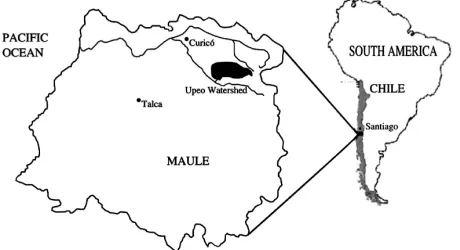
Two methods that define the point of baseflow recession onset were compared using storm hydrograph data for 27 storm events that occurred between 1982-1995 in the Upeo watershed located in the Andes mountain range in central Chile (Figure 1). Three well-known baseflow recession equations were used to determine whether the method we are proposing here, that defines baseflow recession onset as the third inflection point on the logarithmic graph of the falling limb of the storm hydrograph, more accurately models observed data than the most widely used method that defines baseflow onset as the second inflection point on the same graph. Five time intervals were used to modify the recession coefficient in search of a more accurate fit. Results from the coefficient of determination, standard error, Mann-Whit- ney U test, and Bland-Altman test suggest that redefining baseflow recession onset via the proposed approach more accurately models baseflow recession behavior.

Keywords: Baseflow Recession; Hydrograph Separation; Hydrologic Modeling; Recession Analysis; Baseflow Onset

1. Introduction

Predicting the rate of baseflow recession is important to water resource management for areas with Mediterranean climates; as the rate of baseflow decrease (recession) varies little year to year in regions with an extended dry season, recession flow analyses are used to study ground- water systems [1], whose characteristics largely deter- mine the feasibility of land use where options are limited by the availability of water resources (Ponce, 1989).

As direct runoff and baseflow recede at different rates, it is required to model them separately; hydrologists of- ten use surface and subsurface flow models to accom- plish such an objective [2]. Hydrograph separation me- thods are used to determine whether the stream flow present in a channel during a storm event derives from direct runoff or baseflow [3]. However, hydrograph se- paration itself can be considered arbitrary as there is no real basis for the division between surface and subsurface contributions at any given time, as the definition of the hydrograph components themselves (surface, subsurface, and baseflow contributions) are also arbitrarily defined [4,

5]. Regardless, baseflow recession characteristics may still reliably estimate watershed-scale hydrogeological properties [1] and hence justify further study. Baseflow recession models are used to portray the behavior of baseflow and determine minimum water yields and de- pletion rates [6]. Despite their importance, there are sev- eral viewpoints on the effectiveness of baseflow reces- sion models, which often do not accurately model ob-served data.

Several studies worldwide have focused on improving the prediction of baseflow recession. Chapman [7] inves- tigated various algorithms describing baseflow during the precipitation-runoff process and determined that prob- lems arose during the course of hydrograph separation itself. Vogel and Kroll [8] tested six estimators of the baseflow recession constant derived from data for thou- sands of recession hydrographs pertaining to 23 sites in Massachusetts, in the process highlighting how certain assumptions made regarding model error structure af- fected model accuracy.

Figure 1. The lacation of the Upeo watershed within the region of Maule.

widely used method used to date developed by Linsley et al. [9] with the approach we are proposing here (hence- forth referred to as the original and modified approaches

respectively). Using discharge data for a small watershed located in the Andes mountain range of central Chile we compared the two onset point definitions using various baseflow recession equations in order to determine whe- ther the modified approach more accurately models ob- served baseflow behavior.

Site Description

The Upeo is a snow-fed creek that originates in the An- des mountain range of central Chile, running for 126 km before discharging into the Lontué River en route to the Pacific Ocean [10]. Its watershed covers a surface area of 2510 km2 _{and receives close to 1800 mm of precipitation} annually. Annual average flows are estimated at 78.9 m3_·s−1 _[11].

The Chilean government agency in charge of manag- ing the country’s water resources, the Dirección General

de Aguas (DGA), manages a gauging stationat the con-

fluence of the Upeo and the Lontué River (35˚10'23"S lat; 71˚05'28"W long). Using limnograph and discharge curve data from the Upeo Station, storm hydrographs and base- flow recession curves were created for 27 storm events from the period of 1982-1995. Storm events used in this analysis were chosen based on having the most continu- ous and extensive data available for the falling limb of the storm hydrographs.

2. Methods

2.1. Graphical Definition of Baseflow Recession Onset

A storm hydrograph, a graphical representation of the relationship between channel flow versus time during a storm event, is characterized by a rising limb, a peak flow, a falling limb, and a baseflow recession curve [12]. The response of the storm hydrograph is affected by a combination of watershed and climatic characteristics,

which include hydrologic losses and surface runoff char- acteristics, among other variables [3].

The general shape of a storm hydrograph is shown in Figure 2. The most commonly used protocol to separate hydrographs was developed by Linsley et al. [9] and consists of drawing an imaginary line from point A that continues the trajectory of the baseflow recession curve prior to the onset of the storm until peak flow (point B) has been reached. After peak flow is reached, subsurface (seepage) flows are considered to be contributing to chan- nel flow and a second line is drawn to point C, from which point on channel flow is solely comprised of ground- water contributions (baseflow recession).

Baseflow recession onset is identified using data from the falling limb of the storm hydrograph, which is plotted on a logarithmic graph of flow versus time where it pre- sents as a linear graphic distribution with three inflection points. The use of the second inflection point (Point C in Figure 3) to define baseflow recession onset corresponds to the original approach developed by Linsley et al. [9]; the modified approach being proposed here redefines baseflow onset as the third inflection point on the same graph (Point D). Other hydrograph separation method- ologies, such as those proposed by Bedient and Hubert [3] and Viessman and Lewis [5], offer more rough approxi- mations of baseflow recession behavior but were not considered appropriate for the type of analysis used in this study.

2.2. Baseflow Recession Equations

Baseflow recession equations are derived from the base model [3]:

kt

t o

Q Q e (1) where Q0 represents baseflow volume in m3·s−1 at time t0,

Qtis baseflow volume in m3·s−1 at time t, e is the Neper

Figure 3. An example of the falling limb of a storm hydro- graph and its inflection points.

constant, and k is the recession coefficient. The original and modified approaches were compared by defining time t0as either the second (Point C) or third (Point D) inflection point.

The equations used in this comparison were required to accurately reflect the behavior of flow as decreasing as a function of time at the onset of baseflow recession (Pi- zarro, 1993), or in other words satisfy the condition q/dt

< 0 at t0. Widely used models by authors such as Re- menieras [14], Singh [15], and Maidment [12] were con- sidered. However, the following three models were se- lected for use based on their statistical accuracy with observed data (defined as higher R2_{and lower SEE val-} ues):

 





Q t Q t  (2)

 

0 at

Q t _Q e ₍₃₎

 

0 a t

Q t _Q e ₍₄₎

Equation parameters are identical to Equation (1) above, with the exception of alpha (α),which replaces k

as the recession coefficient.

In order to determine if an increase in elapsed time from point t0would help the models to better reflect the observed data, the following five time intervals were chosen to adjust the model parameter of time t: 10, 15, 20, 24, and 48 hours, all of which were used previously with satisfactory results.

Next, the results for the three equations using the ori- ginal and modified approaches were calibrated and vali- dated in comparison with the observed data [15]. We used the coefficient of determination (R2_{) and the stan-} dard error of estimation (SEE) to validate results along with the following statistical tests: the Mann-Whitney U

test, whose central objective is to determine whether or not independent samples come from the same population [16], and the Bland-Altman test, which quantifies the

difference between the observed and modeled data [17]. All statistical analyses were evaluated using a signifi- cance level α = 0.05.

3. Results and Discussion

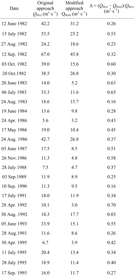
The data for the 27 storm events used in this study along with their corresponding Q0 values for the original and modified approaches are shown in Table 1. The high variability shown in the data made it difficult to develop a precise equation specific to the data.

Table 1. Dates and onset flows using the original and modi- fied approaches for the 27 studied flood events.

Date approach Original

Q0(o) (m3·s−1)

Modified approach Q0(m) (m3·s−1)

Δ = (Q0(o)−Q0(m))/Q0(o) (m3_·s−1₎

12 June 1982 42.2 31.2 0.26

15 July 1982 53.5 25.2 0.53

27 Aug. 1982 24.2 18.6 0.23

12 Sep. 1982 67.0 45.8 0.32

03 Oct. 1982 39.0 15.6 0.60

20 Oct.1982 38.5 26.8 0.30

20 June 1983 14.0 5.2 0.63

06 July 1983 33.3 11.6 0.65

24 Aug. 1983 18.6 15.7 0.16

19 June 1984 13.6 9.8 0.28

24 Apr. 1986 5.6 3.2 0.43

17 May 1986 19.0 10.4 0.45

24 Aug. 1986 42.7 26.8 0.37

03 June 1987 17.5 8.5 0.51

26 Nov.1986 11.3 4.8 0.58

28 July 1988 7.5 4.7 0.37

03 Sep.1989 11.9 8.9 0.25

10 Sep. 1990 11.3 9.5 0.16

17 July 1991 18.0 11.9 0.34

28 Apr. 1992 10.1 3.0 0.70

30 Aug. 1992 18.3 17.7 0.03

05 June 1993 33.9 15.1 0.55

28 Aug.1993 11.6 8.6 0.26

30 Apr. 1995 6.7 3.9 0.42

11 July 1995 20.4 13.4 0.34

28 July 1995 18.9 11.4 0.40

17 Sep. 1995 16.0 11.7 0.27

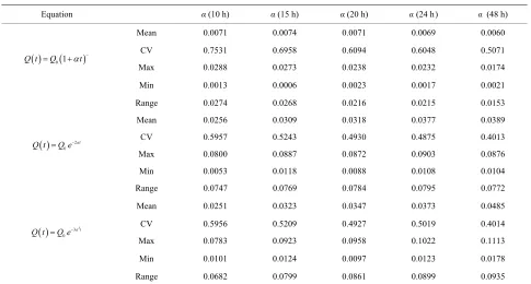
For the original and modified approaches, Equations (3) and (4) both overestimated whereas quadratic Equa- tion (2) slightly underestimated observed flow. For all three models values for the recession coefficient α aver-

aged higher for the original approach than the modified (Tables 2(a) and (b)), which was to be expected as the displacement of Q0 from the second to third inflection point significantly altered the slope of the curve.

Table 2. (a) Recession coefficient values α for the equations using the original approach; (b) Recession coefficient α values for the equations using the modified approach.

(a)

Equation α (10 h) α (15 h) α (20 h) α (24 h) α (48 h)

Mean 0.0071 0.0074 0.0071 0.0069 0.0060

CV 0.7531 0.6958 0.6094 0.6048 0.5071

Max 0.0288 0.0273 0.0238 0.0232 0.0174

  01 

Q t Q t 

 

Min 0.0013 0.0006 0.0023 0.0017 0.0021

Range 0.0274 0.0268 0.0216 0.0215 0.0153

Mean 0.0256 0.0309 0.0318 0.0377 0.0389

CV 0.5957 0.5243 0.4930 0.4875 0.4013

Max 0.0800 0.0887 0.0872 0.0903 0.0876

  2 0

at

Q t _Q e

Min 0.0053 0.0118 0.0088 0.0108 0.0104

Range 0.0747 0.0769 0.0784 0.0795 0.0772

Mean 0.0251 0.0323 0.0347 0.0373 0.0485

CV 0.5956 0.5209 0.4927 0.5019 0.4014

Max 0.0783 0.0923 0.0958 0.1022 0.1113

  ₃3

0 a t

Q t _Q e

Min 0.0101 0.0124 0.0097 0.0123 0.0178

Range 0.0682 0.0799 0.0861 0.0899 0.0935

α = recession coefficient, CV = coefficient of variation.

(b)

Equation α (10 h) α (15 h) α (20 h) α (24 h) α (48 h)

Mean 0.0041 0.0033 0.0031 0.0030 0.0027

CV 0.4348 0.5586 0.4477 0.4197 0.5509

Max 0.0069 0.0085 0.0060 0.0052 0.0053

  01 

Q t Q t 

 

Min 0.0011 0.0002 0.0007 0.0008 0.0007

Range 0.0058 0.0083 0.0053 0.0043 0.0059

Mean 0.0167 0.0169 0.0172 0.0184 0.0207

CV 0.3602 0.4693 0.4223 0.3618 0.4970

Max 0.0269 0.0310 0.0252 0.0271 0.0325

  2 0

at

Q t _Q e

Min 0.0082 0.0034 0.0071 0.0054 0.0024

Range 0.0187 0.0276 0.0184 0.0217 0.0349

Mean 0.0164 0.0179 0.0186 0.0201 0.0254

CV 0.3606 0.4631 0.4236 0.3728 0.4947

Max 0.0263 0.0325 0.0276 0.0307 0.0413

  ₃3

0 a t

Q t _Q e

Min 0.0041 0.0035 0.0032 0.0061 0.0031

Range 0.0222 0.0290 0.0244 0.0246 0.0444

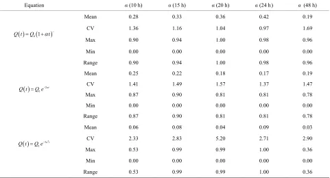
Coefficient of determination values (R2_{) were gener-} ally low for both approaches (Tables 3(a) and (b)), but were relatively higher for the original approach. How-

ever, SEE tended to decrease with an increase in elapsed time for the original approach (Tables 4(a) and (b)), reaching a minimum for Equations (2) and (4) at hour 48;

Table 3. (a) Coefficient of determination R2 values for the equations using the original approach; (b) Coefficient of determi- nation R2 values for the equations using the modified approach.

(a)

Equation α (10 h) α (15 h) α (20 h) α (24 h) α (48 h)

Mean 0.37 0.34 0.30 0.33 0.30

CV 0.98 1.04 1.17 1.11 1.31

Max 0.94 0.95 0.94 0.98 0.95

  01 

Q t Q t 

 

Min 0.00 0.00 0.00 0.00 0.00

Range 0.94 0.95 0.94 0.98 0.95

Mean 0.25 0.25 0.39 0.41 0.56

CV 1.39 1.39 1.01 0.91 3.99

Max 0.91 0.91 0.95 0.98 1.00

  2 0

at

Q t _Q e

Min 0.00 0.00 0.00 0.00 0.00

Range 0.91 0.91 0.95 0.98 1.00

Mean 0.00 0.05 0.03 0.06 0.21

CV - 3.68 3.92 3.26 1.39

Max 0.00 0.77 0.55 0.85 0.87

  ₃3

0 a t

Q t _Q e

Min 0.00 0.00 0.00 0.00 0.00

Range 0.00 0.77 0.55 0.85 0.87

α = recession coefficient, CV = coefficient of variation.

(b)

Equation α (10 h) α (15 h) α (20 h) α (24 h) α (48 h)

Mean 0.28 0.33 0.36 0.42 0.19

CV 1.36 1.16 1.04 0.97 1.69

Max 0.90 0.94 1.00 0.98 0.96

  01 

Q t Q t 

 

Min 0.00 0.00 0.00 0.00 0.00

Range 0.90 0.94 1.00 0.98 0.96

Mean 0.25 0.22 0.18 0.17 0.19

CV 1.41 1.49 1.57 1.37 1.47

Max 0.87 0.90 0.81 0.81 0.78

  2 0

at

Q t _Q e

Min 0.00 0.00 0.00 0.00 0.00

Range 0.87 0.90 0.81 0.81 0.78

Mean 0.06 0.08 0.04 0.09 0.03

CV 2.33 2.83 5.20 2.71 2.90

Max 0.53 0.99 0.99 1.00 0.36

  ₃3

0 a t

Q t _Q e

Min 0.00 0.00 0.00 0.00 0.00

Range 0.53 0.99 0.99 1.00 0.36

Table 4. (a) SEE values for the equations using the original approach; (b) SEE values for the equations using the modified approach.

(a)

Equation α (10 h) α (15 h) α (20 h) α (24 h) α (48 h)

Mean 2.266 2.346 2.165 1.927 1.434

CV 0.728 0.717 0.714 0.686 0.800

Max 7.781 6.861 5.923 5.426 5.071

   2 0 1

Q t Q t 

 

Min 0.377 0.326 0.511 0.279 0.266

Range 7.404 6.534 5.412 5.147 4.804

Mean 4.131 2.633 1.997 0.957 1.017

CV 1.271 0.993 1.026 0.915 0.958

Max 12.857 10.002 6.781 6.540 4.428

  2 0

at

Q t _Q e

Min 0.295 0.263 0.241 0.086 0.091

Range 12.562 9.739 6.540 6.454 4.337

Mean 5.895 4.278 3.483 3.300 1.694

CV 1.058 0.930 0.918 0.881 1.018

Max 29.177 16.434 13.472 11.898 7.749

  ₃3

0 a t

Q t _Q e

Min 1.142 0.546 0.447 0.230 0.113

Range 28.035 15.888 13.025 11.668 7.636

α = recession coefficient, CV = coefficient of variation.

(b)

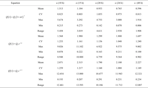
Equation α (10 h) α (15 h) α (20 h) α (24 h) α (48 h)

Mean 1.513 1.184 0.953 0.765 0.596

CV 0.823 0.803 1.053 0.973 0.813

Max 5.674 3.292 4.753 3.008 1.914

   2 0 1

Q t Q t 

 

Min 0.215 0.273 0.142 0.070 0.006

Range 5.458 3.019 4.611 2.938 1.908

Mean 1.568 1.980 1.299 1.880 1.697

CV 1.253 1.161 1.156 1.048 1.240

Max 9.026 11.102 6.922 9.575 9.002

  2 0

at

Q t _Q e

Min 0.078 0.222 0.163 0.211 0.100

Range 8.948 10.800 6.759 9.364 8.902

Mean 2.071 2.315 1.790 2.180 2.227

CV 1.259 1.217 1.160 1.088 1.149

Max 12.654 13.800 10.477 11.943 12.321

  ₃3

0 a t

Q t _Q e

Min 0.193 0.207 0.291 0.231 0.234

Range 12.461 13.593 10.186 11.712 12.087

and for Equation (3) at hour 24. This decrease in accu- racy with an increase in elapsed time is in direct dis- agreement with the R2 _{analysis, which could be explained} by the fact that R2 _{is independent of SEE and only quan-} tifies the variability in the data.

On the other hand, only Equation (2) saw a decrease in

SEE values for an increase in elapsed time using the modified approach. Regardless, all three equations ob- tained smaller SEE values for the modified approach than the original. This, along with the corresponding R2 _values, clearly suggests that the modified approach better adjusts to observed data.

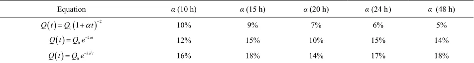
To further the statistical analysis average observed values were compared by obtaining the quotients be- tween SEE and the observed flows for the 27 selected storm events for the respective equation, approach, and time interval. A recession coefficient α value of 48 hours

produced the best results for the original approach, as shown in Tables 5(a) and (b). Only Equation (2) showed an increase in accuracy with a corresponding increase in the amount of elapsed time for the modified approach.

Results from the Mann-Whitney U test are shown in Tables 6(a) and (b), where the percentage of accepted tests for the three equations and five time intervals are tabulated for ease of interpretation. According to the analysis, Equation (3) had the highest number of ac- cepted tests for the original approach, whereas Equation (2) was superior for the modified approach. The modified approach showed the highest acceptance rate for all time intervals and equations analyzed.

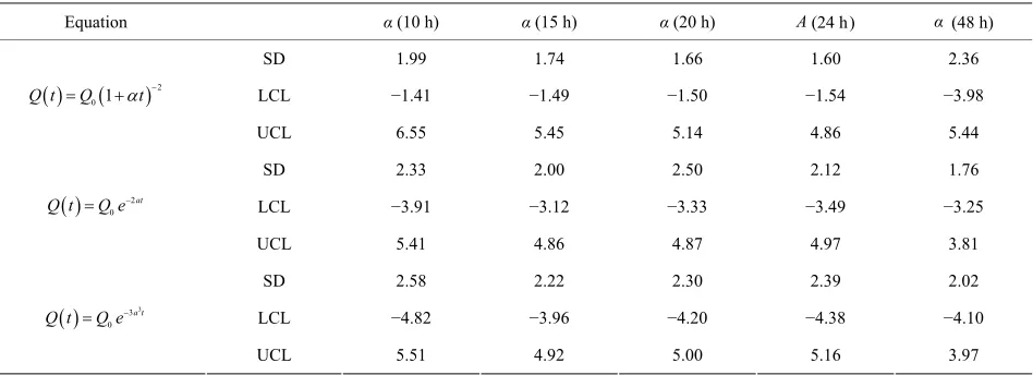
Finally, the results for a comparison between observed and modeled data using the Bland-Altman test are shown in Tables 7(a) and (b). Results indicate that the standard deviations of mean difference are significantly lower for

Table 5. (a) Quotients between SEE and average observed flows for the equations using the original approach; (b) Quotients between SEE and average observed flows for the equations using the modified approach.

(a)

Equation α (10 h) α (15 h) α (20 h) α (24 h) α (48 h)

   2 0 1

Q t Q t 

  20% 22% 20% 19% 15%

  2 0

at

Q t _Q e

32% 20% 15% 15% 8%

  ₃3

0 a t

Q t _Q e _{46% 33% 27% 26% 13%}

α = recession coefficient.

(b)

Equation α (10 h) α (15 h) α (20 h) α (24 h) α (48 h)

   2 0 1

Q t Q t 

  10% 9% 7% 6% 5%

  2 0

at

Q t _Q e

12% 15% 10% 15% 14%

  ₃3

0 a t

Q t _Q e _{16% 18% 14% 17% 18%}

α = recession coefficient.

Table 6. (a) Approval percentages for the Mann-Whitney U test for the equations using the original approach; (b) Approval percentages for the Mann-Whitney U test for the equations using the modified approach.

(a)

Equation α (10 h) α (15 h) α (20 h) α (24 h) α (48 h)

   2 0 1

Q t Q t  14.8% 14.8% 3.7% 14.8% 22.2%

  2 0

at

Q t _Q e

7.4% 3.7% 14.8% 14.8% 59.3%

  ₃3

0 a t

Q t _Q e _{0.0% 0.0% 0.0% 0.0% 22.2%}

α = recession coefficient.

(b)

Equation α (10 h) α (15 h) α (20 h) α (24 h) α (48 h)

   2 0 1

Q t Q t 

  25.9% 22.2% 29.6% 55.6% 37.0%

  2 0

at

Q t _Q e

22.2% 14.8% 18.5% 25.9% 60.0%

  ₃3

0 a t

Q t _Q e _{11.1% 3.7% 11.1% 18.5% 52.0%}

Table 7. (a) Results for the Bland-Altman test applied to the equations using the original approach; (b) Results for the Bland-Altman test applied to the equations using the modified approach.

(a)

Equation α (10 h) α (15 h) α (20 h) α (24 h) α (48 h)

SD 2.65 2.38 1.96 1.54 0.96

LCL −4.73 −3.68 −2.69 −1.94 −1.13

   2 0 1

Q t Q t 

 

UCL 5.87 5.85 5.14 4.22 2.71

SD 5.67 3.50 3.02 2.86 2.58

LCL −14.75 −8.86 −7.51 −7.04 −6.05

  2 0

at

Q t _Q e

UCL 7.93 5.15 4.56 4.40 4.28

SD 5.89 3.72 2.98 2.68 2.29

LCL −17.25 −11.33 −9.31 −8.41 −7.06

  ₃3

0 a t

Q t _Q e

UCL 6.33 3.55 2.59 2.30 2.10

α = recession coefficient, SD = standard deviation, LCL and UCL= lower and upper confidence limits, respectively.

(b)

Equation α (10 h) α (15 h) α (20 h) Α(24 h) α (48 h)

SD 1.99 1.74 1.66 1.60 2.36

LCL −1.41 −1.49 −1.50 −1.54 −3.98

   2 0 1

Q t Q t 

 

UCL 6.55 5.45 5.14 4.86 5.44

SD 2.33 2.00 2.50 2.12 1.76

LCL −3.91 −3.12 −3.33 −3.49 −3.25

  2 0

at

Q t _Q e

UCL 5.41 4.86 4.87 4.97 3.81

SD 2.58 2.22 2.30 2.39 2.02

LCL −4.82 −3.96 −4.20 −4.38 −4.10

  ₃3

0 a t

Q t _Q e

UCL 5.51 4.92 5.00 5.16 3.97

α = recession coefficient, SD = standard deviation, LCL and UCL = lower and upper confidence limits, respectively.

the modified approach, which is further supported by the confidence interval analysis. Similarly, data dispersion around the mean values was more uniform for the modi- fied approach.

4. Conclusions and Recommendations

On the basis of the completed statistical analyses for all three selected equations, in particular the results of the Mann-Whitney U test, we conclude that the modified approach more accurately predicts baseflow recession behavior; or, that model accuracy is improved by defin- ing the onset of baseflow recession as the third inflection point of the logarithmic graph of the falling limb of the storm hydrograph. Results of this study question the fea- sibility of continuing to use the current hydrograph sepa- ration procedure proposed in 1949 by Linsley et al. [9]. We strongly recommend considering this new modified

approach for future studies.

Of the three selected and analyzed equations, the qua- dratic model Equation (2) offered the best modeling re- sults. However, the authors recommend continuing to test other equations to improve even more the estimation of baseflow recession, as well as the use of more statistical parameters besides the coefficient of determination R2_.

REFERENCES

[1] M. Manga, “Origin of Post Seismic Stream Flow Changes Inferred from Baseflow and Magnitude-Distance Rela- tions,” Geophysical Research Letters, Vol. 28, No. 10, 2001, pp. 2133-2136.

Analysis,” 3rd Edition,Prentice Hall, Englewood Cliffs, 2002.

[4] R. Linsley and M. Kohler, “Hydrology for Engineers,” 2nd Edition, McGraw-Hill, New York, 1975.

[5] W. Viessman and G. Lewis, “Introduction to Hydrology,” 5th Edition, Prentice Hall, Engelwood Cliffs, 2003. [6] G. N. Martin, “Characterization of Simple Exponential

Baseflow Recessions,” New Zealand Journal of Hydrol- ogy, Vol. 12, No. 1, 1973, pp. 57-62.

[7] T. Chapman, “A Comparison of Algorithms for Stream Flow Recession and Baseflow Separation,” Hydrological Processes, Vol. 13, No. 5, 1999, pp. 701-714.

[8] R. Vogel and C. Kroll, “Estimation of Baseflow Reces- sion Constants,” Water Resources Management (Nether- lands), Vol. 10, No. 4, 1996, pp. 303-320.

[9] R. Linsley, M. Kohler and J. Paulhus, “Applied Hydrol- ogy,” McGraw-Hill, New York, 1949.

[10] H. Niemeyer and P. Cereceda, “Hidrografía. Geografía de

Chile. Tomo VIII,” Instituto Geográfico Militar de Chile, Santiago, 1983.

[11] Dirección General de Aguas (DGA), “Estudio del Mapa Hidrogeológico Nacional,” 1986.

[12] D. Maidment, “Handbook of Hydrology,” McGraw-Hill, New York, 1993.

[13] V. Chow, D. Maidment and L. W. Mays, “Applied Hy- drology,”McGraw-Hill, New York, 1949.

[14] G. Remenieras, “Tratado de Hidrología Aplicada. Primera Edición Española,” Técnicos Asociados S.A. Barcelona, Spain, 1971.

[15] V. Singh, “Hydrologic Systems: Rainfall-Runoff Model- ing,” Prentice Hall, Englewood Cliffs, 1988.

[16] R. Mason and D. Lind, “Statistical Techniques in Busi- ness and Economics,” 8th Edition, University of Toledo, Ohio, 1998.

[17] J. Bland and D. Altman, “Measuring Agreement in Me- thod Comparison Studies,” Statistical Methods in Medical Research, Vol. 8, No. 2, 1999, pp. 135-160.