AppliedMathematics, 2013, 4, 1503-1511
Published Online November 2013 (http://www.scirp.org/journal/am) http://dx.doi.org/10.4236/am.2013.411203
The Sum and Difference of Two Constant Elasticity of
Variance Stochastic Variables
Chi-Fai Lo
Department of Physics, Institute of Theoretical Physics, The Chinese University of Hong Kong, Hong Kong, China
Email: [email protected]
Received August 20,2013; revised September 20, 2013; accepted September 27, 2013
Copyright © 2013 Chi-Fai Lo. This is an open access article distributed under the Creative Commons Attribution License, which permits unrestricted use, distribution, and reproduction in any medium, provided the original work is properly cited.
ABSTRACT
We have applied the Lie-Trotter operator splitting method to model the dynamics of both the sum and difference of two
correlated constant elasticity of variance (CEV) stochastic variables. Within the Lie-Trotter splitting approximation,
both the sum and difference are shown to follow a shifted CEV stochastic process, and approximate probability
distri-butions are determined in closed form. Illustrative numerical examples are presented to demonstrate the validity and
accuracy of these approximate distributions. These approximate probability distributions can be used to valuate
two-asset options, e.g. spread options and basket options, where the CEV variables represent the forward prices of the
underlying assets. Moreover, we believe that this new approach can be extended to study the algebraic sum of
N
CEV
variables with potential applications in pricing multi-asset options.
Keywords:
Constant Elasticity of Variance Stochastic Variables; Probability Distribution Functions; Backward
Kolmogorov Equation; Lie-Trotter Splitting Approximation
1. Introduction
Recently Lo [1] proposed a new simple approach to tackle
the long-standing problem: “
Given
two
correlated
log-normal
stochastic
variables
,
what
is
the
stochastic
dy-namics
of
the
sum
or
difference
of
the
two
variables
?”; or
equivalently, “
What
is
the
probability
distribution
of
the
sum
or
difference
of
two
correlated
lognormal
stochastic
variables
?” The solution to this problem has wide
appli-cations in many fields including financial modelling,
actu-arial sciences, telecommunications, biosciences and
phys-ics [2-15]. By means of the Lie-Trotter operator splitting
method [16], Lo showed that both the sum and difference
of two correlated lognormal stochastic processes could
be approximated by a shifted lognormal stochastic
proc-ess, and approximate probability distributions were
de-termined in closed form. Unlike previous studies which
treat the sum and difference in a separate manner [2-5,
8,13,15,17-27], Lo’s method provides a new unified
ap-proach to model the dynamics of both the sum and
dif-ference of the two stochastic variables. In addition, in
terms of the approximate solutions, Lo presented an
ana-lytical series expansion of the exact solutions, which can
allow us to improve the approximation systematically.
In this communication we extend Lo’s approach to
study the dynamics of both the sum and difference of two
correlated constant elasticity of variance (CEV)
stochas-tic processes. The CEV process was first proposed by
Cox and Ross [28] as an alternative to the lognormal
stochastic movements of stock prices in the Black-
Scholes model. The CEV process, which is defined by
the stochastic differential equation
2
2. Lie-Trotter Operator Splitting Method
We consider two CEV stochastic variables
1and
2,
which are described by the stochastic differential equa-
tions:
S S
2
dSi
iSi dZi , i1,2 2(2)
for
0
. Here
dZidenotes a standard Weiner
process associated with
, and the two Weiner
proc-esses are correlated as
1 2i
S
d dZ Z
dt1
. Without loss of
generality, we also assume that
2. The joint
prob-ability distribution function
P S S t
1, 2, 10,S20,t0
of the
two correlated CEV variables obeys the backward
Kol-mogorov equation [42-45]
;S
1 2 10 20 0
0
ˆ , , ; , , 0
L P S S t S S t
t
(3)
where
2 2
2 2 2
1 10 2 1 2 10 20
10 20 10
2 2
2 20 2
20 1 ˆ 2 1 , 2
L S S S
S S S S S
(4)
subject to the boundary condition
1, 2, ; 10, 20,0
1 10
2 20P S S t S S t t
S S
S S
.
(5)
This joint probability distribution function tells us how
probable the two CEV variables assume the values
and
2at time
0, provided that their values at
are given by
10and
20. Once
is found, the probability distribution of the sum or
dif-ference, namely
1 2, of the two correlated
CEV variables can be obtained by evaluating the integral
1 S 0 t 0 ,t
S tt
S S
S S
1, 2, ; 10, 20P S S t S S
S
10 20 0
1 2 1 2 10 20 0 1 2 0 0
, ; , ,
d d , , ; , , .
P S t S S t
S S P S S t S S t
S S S
(6)
Unfortunately, the joint probability distribution function
is not available in closed form, except for the case of
0
. Hence, we must resort to numerical methods, e.g.
the finite-difference method or Monte Carlo simulation.
Nevertheless, the numerically exact solution does not
provide any information about the stochastic dynamics of
the sum or difference explicitly.
It is observed that the probability distribution of the
sum or difference of the two correlated CEV variables,
i
.
e
.
P S
, ;
t S
10,
S
20,
t
0
, also satisfies the same
back-ward Kolmogorov equation given in Equation (3), but
with a different boundary condition [43]
, ;
10,
20,
0
10 20
.
P S
t S
S
t
t
S
S
S
(7)
To solve for
, ;
10,
20,
0
0 0 0
0
ˆ
ˆ
ˆ
, ;
,
,
0
L
L
L
P S
t S
S
t
t
0
(8)
where
2 2
2
0 0 0
1 1 2
0 0 2 2 0 2 2 0 0 1
ˆ 1 2 1
2 2
1
S S S
L S S S S S
(9)
2 2 20 0 0
1 1 2
0 0 2 2 0 2 2 0 0 1
ˆ 1 2 1
2 2
1
S S S
L S S S S S
(10)
2 2 0 0 2 0 00 1 2
0 0
ˆ
2 2
S S S S
L S S
(11)
2 21 2 2 1 2.
(12)
The corresponding boundary condition now becomes
, ; 0, 0,0
0 .P S t S S t
t
S
S
(13)
Accordingly, the formal solution of Equation (8) is
readily given by
0 0 0
0 0 0
, ; , ,
ˆ ˆ ˆ
exp .
P S t S S t
t t L L L
S S
(14)
Since the exponential operator
0 ˆ ˆ0 ˆ
exp tt LL L
is difficult to evaluate, we
apply the Lie-Trotter operator splitting method
1to
ap-*Suppose that one needs to exponentiate an operator Cˆ which can be
split into two different parts, namely ˆA and ˆB. For simplicity, let us assume that Cˆ Aˆ Bˆ, where the exponential operator exp
Cˆ is difficult to evaluate but exp
Aˆ and exp
Bˆ are either solvable or easy to deal with. Under such circumstances the exponential operator
ˆexp C , with being a small parameter, can be approximated by the Lie-Trotter splitting formula (Trotter, 1959):
ˆ
ˆ ˆ
2exp C exp A expB O .
This can be seen as the approximation to the solution at t of the equation dYˆdt
AˆB Yˆ ˆ
by a composition of the exact solutions of the equations dYˆdtAYˆˆ and dYˆ dtBYˆ
P S
t S
S
t
, we first rewrite the
backward Kolmogorov equation in terms of the new
variables
S
0S
10S
2as
ˆ at time
t .
1505
proximate the operator by [16,46-49]
0
0
0
ˆLT exp ˆ exp ˆ ˆ ,
O tt L tt L L
(15)
and obtain an approximation to the formal solution
, ;
0,
0,
0
P S
t S
S
t
, namely
0 0 0
0 0
, ; , ,
ˆ exp ˆ
LT LT
P S t S S t
O
S S t t L S S
0
(16)
where the relation
0 ˆ0 ˆ
0
0exp tt L L
SS
SSis
util-ized. For
S
0S
0
21
, which is normally valid unless
10
and
20are both close to zero, the operators
S
S
L
ˆ
and
L
ˆ
can be approximately expressed as
2 2 0 2 0
1
ˆ
2
L
S
S
(17)
in terms of the two new variables:
2 2 1 2 0 0 2
S
S
S
0 (18)
2 0 0 2 2 01 2
.
S
S
S
(19)
Here the parameters
and
are defined by
2
2
(20)
2
2 2
1 1 2 .
2
(21)
Obviously, both
S
and
S
are CEV random
vari-ables defined by the stochastic differential equations
2
dS
S dZ,(22)
and their closed-form probability distribution functions
are given by
CEV 0 01 2 1 2 2 2 2
0 0
1 2
2 2 2
0 0 2 2 0 2 2 0
, ;
,
2
4
2
2
2
exp
2
f
S
t S
t
S
S
S S
I
t
t
t
t
S
S
t
t
(23)
for
0, where
denotes the modified Bessel
function of order
t
t
I
. As a result, it can be inferred that
within the Lie-Trotter splitting approximation both
S
and
S
are governed by a shifted CEV process. It
should be noted that for the Lie-Trotter splitting
ap-proximation to be valid,
2
t
t
0
needs to be small.
3. Illustrative Numerical Examples
In
Figure 1
we plot the approximate closed-form
prob-ability distribution function of the sum
of two
un-correlated CEV variables (
i
.
e
.
S
0
) given in Equation
(23) for different values of the input parameters. We start
with
S
10
110
,
S
20
105
,
10.5
and
20.3
in
Figure 1(a)
. Then, in order to examine the effect of
20,
we decrease its value to
in
Figure 1(b)
and to 65 in
Figure 1(c)
. In
Figures 1(d)
-
(f)
we repeat the same
investigation with a new set of values for
1S
85
and
2,
namely
10.3
and
20.2
. Without loss of
gener-ality, we set
t
t
01
for simplicity. The (numerically)
exact results which are obtained by numerical
integra-tions are also included for comparison. It is clear that the
proposed approximation can provide accurate estimates
for the exact values.
In order to have a clearer picture of the accuracy, we
plot the corresponding errors of the estimation in
Figure
2
. We can easily see that major discrepancies appear
around the peak of the probability distribution function
and that the estimation deteriorates as the elasticity
pa-rameter
increases. It should be noted that the
pro-posed approximation is exact in the special case of
0
,
i
.
e
. the Ornstein-Uhlenbeck model. We also
observed that the errors increase with the ratio
S
0S
0
and
2(or equivalently,
1and
2) as expected.
Next, we apply the same sequence of analysis to the
approximate closed-form probability distribution
func-tion of the difference
S
given in Equation (23).
Simi-lar observations about the accuracy of the proposed
ap-proximation can be made for the difference
S
, too (see
Figures 3
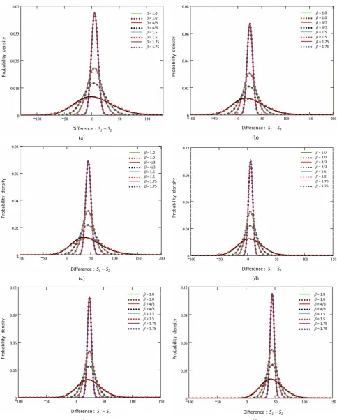
and
4
).
4. Conclusion
[image:3.595.55.290.80.515.2](a) (b)
(c) (d)
[image:4.595.91.505.80.681.2]
(e) (f)
Figure 1. Probability density vs. S1 + S2: the dotted lines denote the distributions of the approximate shifted CEV process, and
the solid lines show the exact results. (a) S10 = 110, S20 = 105, σ1 = 0.5 and σ2 = 0.3; (b) S10 = 110, S20 = 85, σ1 = 0.5 and σ2 = 0.3;
(c) S10 = 110, S20 = 65, σ1 = 0.5 and σ2 = 0.3; (d) S10 = 110, S20 = 105, σ1 = 0.3 and σ2 = 0.2; (e) S10 = 110, S20 = 85, σ1 = 0.3 and σ2
1507
(a) (b)
(c) (d)
[image:5.595.59.539.87.688.2]
(e) (f)
Figure 2. Error vs. S1 + S2: the error is calculated by subtracting the approximate estimate from the exact result. (a) S10 =
110, S20 = 105, σ1 = 0.5 and σ2 = 0.3; (b) S10 = 110, S20 = 85, σ1 = 0.5 and σ2 = 0.3; (c) S10 = 110, S20 = 65, σ1 = 0.5 and σ2 = 0.3; (d)
S10 = 110, S20 = 105, σ1 = 0.3 and σ2 = 0.2; (e) S10 = 110, S20 = 85, σ1 = 0.3 and σ2 = 0.2; (f) S10 = 110, S20 = 65, σ1 = 0.3 and σ2 =
(a) (b)
(c) (d)
[image:6.595.56.539.79.681.2]
(e) (f)
Figure 3. Probability density vs. S1−S2: the dotted lines denote the distributions of the approximate shifted CEV process, and
the solid lines show the exact results. (a) S10 = 110, S20 = 105, σ1 = 0.5 and σ2 = 0.3; (b) S10 = 110, S20 = 85, σ1 = 0.5 and σ2 = 0.3;
(c) S10 = 110, S20 = 65, σ1 = 0.5 and σ2 = 0.3; (d) S10 = 110, S20 = 105, σ1 = 0.3 and σ2 = 0.2; (e) S10 = 110, S20 = 85, σ1 = 0.3 and σ2
1509
(a) (b)
(c) (d)
[image:7.595.56.541.80.686.2]
(e) (f)
Figure 4. Error vs. S1−S2: the error is calculated by subtracting the approximate estimate from the exact result. (a) S10 =
110, S20 = 105, σ1 = 0.5 and σ2 = 0.3; (b) S10 = 110, S20 = 85, σ1 = 0.5 and σ2 = 0.3; (c) S10 = 110, S20 = 65, σ1 = 0.5 and σ2 = 0.3; (d)
S10 = 110, S20 = 105, σ1 = 0.3 and σ2 = 0.2; (e) S10 = 110, S20 = 85, σ1 = 0.3 and σ2 = 0.2; (f) S10 = 110, S20 = 65, σ1 = 0.3 and σ2 =
algebraic sum of
N
CEV variables with potential
applica-tions in pricing multi-asset opapplica-tions.
REFERENCES
[1] C. F. Lo, “The Sum and Difference of Two Lognormal
Random Variables,” Journal of Applied Mathematics,
Vol. 2012, 2012, Article ID: 838397. http://dx.doi.org/10.1155/2012/838397
[2] L. Fenton, “The Sum of Lognormal Probability
Distribu-tions in Scatter Transmission Systems,” IRETransactions onCommunicationsSystems, Vol. 8, No. 1, 1960, pp. 57- 67. http://dx.doi.org/10.1109/TCOM.1960.1097606
[3] J. I. Naus, “The Distribution of the Logarithm of the Sum
of Two Lognormal Variates,” Journal ofthe American
StatisticalAssociation, Vol. 64, No. 326, 1969, pp. 655-
659. http://dx.doi.org/10.1080/01621459.1969.10501004
[4] M. A. Hamdan, “The Logarithm of the Sum of Two
Cor-related Lognormal Variates,” Journal of the American
StatisticalAssociation, Vol. 66, No. 333, 1971, pp. 105-
106. http://dx.doi.org/10.1080/01621459.1971.10482229
[5] C. L. Ho, “Calculating the Mean and Variance of Power
Sums with Two Lognormal Components,” IEEE
Trans-actionsonVehicularTechnology, Vol. 44, No. 4, 1995, pp. 756-762. http://dx.doi.org/10.1109/25.467959
[6] M. A. Milevsky and S. E. Posner, “Asian Options, the
Sum of Lognormals, and the Reciprocal Gamma Distri-bution,” JournalofFinancialandQuantitativeAnalysis, Vol. 33, No. 3, 1998, pp. 409-422.
http://dx.doi.org/10.2307/2331102
[7] J. Dhaene, M. Denuit, M. J. Goovaerts, R. Kaas and D.
Vyncke, “The Concept of Comonotonicity in Actuarial Science and Finance: Applications,” Insurance: Mathe-maticsandEconomics, Vol. 31, No. 2, 2002, pp. 133-161. http://dx.doi.org/10.1016/S0167-6687(02)00135-X
[8] R. Carmona and V. Durrleman, “Pricing and Hedging
Spread Options,” SIAMReview, Vol. 45, No. 4, 2003, pp.
627-685. http://dx.doi.org/10.1137/S0036144503424798
[9] J. H. Graham, K. Shimizu, J. M. Emlen, D. C. Freeman
and J. Merkel, “Growth Models and the Expected
Distri-bution of Fluctuating Asymmetry,” BiologicalJournalof
theLinneanSociety, Vol. 80, No. 1, 2003, pp. 57-65. http://dx.doi.org/10.1046/j.1095-8312.2003.00220.x
[10] M. Romeo, V. Da Costa and F. Bardon, “Broad
Distribu-tion Effects in Sums of Lognormal Random Variables,”
EuropeanPhysicalJournalB, Vol. 32, No. 4, 2003, pp. 513-525. http://dx.doi.org/10.1140/epjb/e2003-00131-6
[11] D. Dufresne, “The Log-Normal Approximation in
Finan-cial and Other Computations,” AdvancesinApplied Prob-ability, Vol. 36, No. 3, 2004, pp. 747-773.
http://dx.doi.org/10.1239/aap/1093962232
[12] S. Vanduffel, T. Hoedemakers and J. Dhaene,
“Compar-ing Approximations for Risk Measures of Sums of Non-
Independent Lognormal Random Variables,” NorthAme-
ricanActuarialJournal, Vol. 9, No. 4, 2005, pp. 71-82.
[13] J. Wu, N. B. Mehta and J. Zhang, “Flexible Lognormal
Sum Approximation Method,” ProceedingsofIEEEGlobal
TelecommunicationsConference (GLOBECOM’05), Vol.
6, 2005, pp. 3413-3417.
[14] A. Kukush and M. Pupashenko, “Bounds for a Sum of
Random Variables under a Mixture of Normals,” Theory
ofStochasticProcesses, Vol. 13, No. 29, 2007, pp. 82-97.
[15] X. Gao, H. Xu and D. Ye, “Asymptotic Behavior of Tail
Density for Sum of Correlated Lognormal Variables,”
In-ternational Journal of Mathematics and Mathematical Sciences, Vol. 2009, 2009, Article ID: 630857.
[16] H. F. Trotter, “On the Product of Semi-Groups of
Opera-tors,” ProceedingsoftheAmericanMathematicalSociety, Vol. 10, No. 4, 1959, pp. 545-551.
http://dx.doi.org/10.1090/S0002-9939-1959-0108732-6
[17] N. C. Beaulieu and F. Rajwani, “Highly Accurate Simple
Closed-Form Approximations to Lognormal Sum
Distri-butions and Densities,” IEEE Communications Letters,
Vol. 8, No. 12, 2004, pp. 709-711.
http://dx.doi.org/10.1109/LCOMM.2004.837657
[18] C. L. J. Lam and T. Le-Ngoc, “Estimation of Typical
Sum of Lognormal Random Variables Using Log-Shifted
Gamma Approximation,” IEEECommunicationsLetters,
Vol. 10, No. 4, 2006, pp. 234-235.
http://dx.doi.org/10.1109/LCOMM.2006.1613731
[19] L. Zhao and J. Ding, “Least Squares Approximations to
Lognormal Sum Distributions,” IEEE Transactions on
VehicularTechnology, Vol. 56, No. 2, 2007, pp. 991-997. http://dx.doi.org/10.1109/TVT.2007.891467
[20] N. B. Mehta, J. Wu, A. F. Molisch and J. Zhang,
“Ap-proximating a Sum of Random Variables with a
Log-normal,” IEEE Transactions on Wireless
Communica-tions, Vol. 6, No. 7, 2007, pp. 2690-2699. http://dx.doi.org/10.1109/TWC.2007.051000
[21] S. Borovkova, F. J. Permana and H. V. D. Weide, “A
Closed Form Approach to the Valuation and Hedging of Basket and Spread Options,” TheJournalofDerivatives, Vol. 14, No. 4, 2007, pp. 8-24.
http://dx.doi.org/10.3905/jod.2007.686420
[22] D. Dufresne, “Sums of Lognormals,” ActuarialResearch
ConferenceProceedings, Regina, 14-16 August 2008.
[23] Q. T. Zhang and S. H. Song, “A Systematic Procedure for
Accurately Approximating Lognormal-Sum Distributions,”
IEEETransactionsonVehicularTechnology, Vol. 57, No. 1, 2008, pp. 663-666.
http://dx.doi.org/10.1109/TVT.2007.905611
[24] T. R. Hurd and Z. Zhou, “A Fourier Transform Method
for Spread Option Pricing,” SIAM JournalofFinancial
Mathematics, Vol. 1, No. 1, 2010, pp. 142-157. http://dx.doi.org/10.1137/090750421
[25] X. Li, V. D. Chakravarthy and Z. Wu, “A
Low-Com-plexity Approximation to Lognormal Sum Distributions
via Transformed Log Skew Normal Distribution,” IEEE
Transactions on Vehicular Technology, Vol. 60, No. 8, 2011, pp. 4040-4045.
http://dx.doi.org/10.1109/TVT.2011.2163652
[26] N. C. Beaulieu, “An Extended Limit Theorem for
Corre-lated Lognormal Sums,” IEEE Transactionson
Commu-nications, Vol. 60, No. 1, 2012, pp. 23-26.
http://dx.doi.org/10.1109/TCOMM.2011.091911.110054
En-1511
hance the BPW Model for the Pricing of Basket and Spread Options,” TheJournalofDerivatives, Vol. 19, No. 3, 2012, pp. 77-82.
http://dx.doi.org/10.3905/jod.2012.19.3.077
[28] J. C. Cox and S. A. Ross, “The Valuation of Options for
Alternative Stochastic Processes,” Journal of Financial
Economics, Vol. 3, No. 1-2, 1976, pp. 145-166. http://dx.doi.org/10.1016/0304-405X(76)90023-4
[29] J. C. Cox, “The Constant Elasticity of Variance Option
Pricing Model,” JournalofPortfolio Management, Vol.
23, 1996, pp. 15-17.
[30] C. F. Lo, P. H. Yuen and C. H. Hui, “Constant Elasticity
of Variance Option Pricing Model with Time-Dependent
Parameters,” International Journal of Theoretical and
AppliedFinance, Vol. 3, No. 4, 2000, pp. 661-674. http://dx.doi.org/10.1142/S0219024900000814
[31] D. Davydov and V. Linetsky, “The Valuation and
Hedg-ing of Barrier and Lookback Option under the CEV Proc-ess,” ManagementScience, Vol. 47, 2001, pp. 949-965. http://dx.doi.org/10.1287/mnsc.47.7.949.9804
[32] J. Detemple and W. D. Tian, “The Valuation of American
Options for a Class of Diffusion Processes,” Management Science, Vol. 48, No. 7, 2002, pp. 917-937.
http://dx.doi.org/10.1287/mnsc.48.7.917.2815
[33] C. Jones, “The Dynamics of the Stochastic Volatility:
Evidence from Underlying and Options Markets,”
Jour-nalofEconometrics, Vol. 116, No. 1-2, 2003, pp. 181-
224. http://dx.doi.org/10.1016/S0304-4076(03)00107-6
[34] M. Widdicks, P. W. Duck, A. D. Andricopoulos and D. P.
Newton, “The Black-Scholes Equation Revisited: Asymp-totic Expansions and Singular Perturbations,” Mathemati-calFinance, Vol. 15, No. 2, 2005, pp. 373-391.
http://dx.doi.org/10.1111/j.0960-1627.2005.00224.x
[35] J. Xiao, H. Zhai and C. Qin, “The Constant Elasticity of
Variance (CEV) Model and the Legendre Transform— Dual Solution for Annuity Contracts,” Insurance: Mathe-maticsandEconomics, Vol. 40, 2007, pp. 302-310. http://dx.doi.org/10.1016/j.insmatheco.2006.04.007
[36] Y. L. Hsu, T. I. Lin and C. F. Lee, “Constant Elasticity of Variance (CEV) Option Pricing Model: Integration and
Detailed Derivation,” MathematicsandComputersinSi-
mulation, Vol. 79, No. 1, 2008, pp. 60-71. http://dx.doi.org/10.1016/j.matcom.2007.09.012
[37] R. R. Chen, C. F. Lee and H. H. Lee, “Empirical Perfor-
mance of the Constant Elasticity Variance Option Pricing
Model,” ReviewofPacificBasinFinancialMarketsand
Policies, Vol. 12, No. 2, 2009, pp. 1-41. http://dx.doi.org/10.1142/S0219091509001605
[38] J. Gao, “Optimal Portfolios for DC Pension Plans under a
CEV Model,” Insurance: Mathematics and Economics,
Vol. 44, No. 3, 2009, pp. 479-490.
http://dx.doi.org/10.1016/j.insmatheco.2009.01.005
[39] M. Gu, Y. Yang, S. Li and J. Zhang, “Constant Elasticity
of Variance Model for Proportional Reinsurance and In-
vestment Strategies,” Insurance: Mathematics and Eco-
nomics, Vol. 46, No. 3, 2010, pp. 9-18.
[40] X. Lin and Y. Li, “Optimal Reinsurance and Investment
for a Jump Diffusion Risk Process under the CEV Model,”
NorthAmericanActuarialJournal, Vol. 15, No. 3, 2011, pp. 417-431.
http://dx.doi.org/10.1080/10920277.2011.10597628
[41] H. Zhao and X. Rong, “Portfolio Selection Problem with
Multiple Risky Assets under the Constant Elasticity of
Variance Model,” Insurance: MathematicsandEconom-
ics, Vol. 50, No. 1, 2012, pp. 179-190.
http://dx.doi.org/10.1016/j.insmatheco.2011.10.013
[42] J. E. Ingersoll, “Theory of Financial Decision Making,”
Rowman & Littlefield Publishers, Lanham, 1987.
[43] D. R. Cox and H. D. Miller, “Theory of Stochastic Proc-
esses,” Chapman & Hall/CRC, London, 2001.
[44] J. Baz and G. Chacko, “Financial Derivatives: Pricing,
Applications and Mathematics,” Cambridge University Press, Cambridge, 2009.
[45] G. W. Gardiner, “Handbook of Stochastic Methods for
Physics, Chemistry and the Natural Sciences,” Springer, Berlin, 2004.
[46] H. F. Trotter, “Approximation of Semi-Groups of Opera-
tors,” Pacific Journal of Mathematic, Vol. 8, No. 4, 1958, pp. 887-919. http://dx.doi.org/10.2140/pjm.1958.8.887
[47] M. Suzuki, “Decomposition Formulas of Exponential
Operators and Lie Exponentials with Some Applications
to Quantum Mechanics and Statistical Physics,” Journal
of Mathematical Physics, Vol. 26, No. 4, 1985, pp. 601- 612. http://dx.doi.org/10.1063/1.526596
[48] A. N. Drozdov and J. J. Brey, “Operator Expansions in
Stochastic Dynamics,” Physical Review E, Vol. 57, No. 2, 1998, pp. 1284-1289.
http://dx.doi.org/10.1103/PhysRevE.57.1284
[49] N. Hatano and M. Suzuki, “Finding Exponential Product
Formulas of Higher Orders,” Lecture Notes in Physics,