Munich Personal RePEc Archive
A Non-Parametric Approach to Spatial
Causality
Herrera Gómez, Marcos and Ruiz Marín, Manuel and Mur
Lacambra, Jesús and Paelinck, Jean
2010
Online at
https://mpra.ub.uni-muenchen.de/36768/
A Non-Parametric Approach to Spatial Causality
Marcos Herrera(*) Manuel Ruiz(**) Jesús Mur(*) Jean Paelinck(***)
(*) Department of Economic Analysis. University of Zaragoza. E-mail: [email protected]; [email protected]
(**) Department of Quantitative Methods and Computing. Politechnical University of Cartagena.
E-mail: [email protected]
(***) School of Public Policy. George Mason University. E-mail: [email protected]
Abstract
The purpose of this paper is to show the capacity of a new non-parametric test based on symbolic entropy and symbolic dynamics to deal with the detection of linear and non-linear spatial causality. The good performance of the new test in detecting spatial causality and causal weighting matrix is notable and gives rise to an expectation that it may form a adequate tool for constructive specification searches.
Keywords: Causality; Spatial Dependence; Spatial Weight Matrices.
1
Introduction
Detection of cause-effects relationships among variable has been one of the fundamental questions of most part of natural or social sciences, including Economics. The bibliometric study of Hoover (2004, p.4) is very illustrative: 70% of the articles in the JSTORarchives published in 2001, contain words ‘in a causal family (“cause”, “causes”, “causal”, “causally” or “causality”)’. The percentage increases up to the 80% if the search is restricted only to econometric articles. It is clear that causality is one of the leading topics in mainstream Economics and Econometrics. In contrast, the Index of Lesage and Pace (2009) textbook on Spatial Econometrics contains almost 1,000 headwords, none of which is related to the Hoover’s causal family. Exactly the same can be said with respect to other textbooks published in the field such as Paelinck and Klaassen (1979), Anselin (1988), Upton and Fingleton (1985), Anselin and Florax (1995), Tiefelsdorf (2000), Griffith (2003), Anselin, Florax and Rey (2004), Getis, Mur and Zoller (2004) or Arbia (2006). This silence is striking and hardly justifiable.
The traditional approach to causality (i.e., Suppes, 1970) insists in the idea of temporal precedence: the cause must occur before the effect. Granger (1980) adds a second fundamental clause: the variable supposed to be the cause must contain information about the effect that is unique, and is in no other variable. The consequence is that the causal variable should help to forecast the effect variable, leading to the concept of ‘incremental predictability’ as a quantifiable, and successful, measure of causality. This is the same idea made by Wiener (1956): ‘For two simultaneously measured signals, if we can predict the first signal better by using the past information from the second one than by using the information without it, then we call the second signal causal to the first one’.
In a typical spatial econometric problem we have a single cross-section collection of contemporaneous data, without time perspective. Forecasting is not a hot topic here where, put it very rude, the main problem is explaining the spatial distribution of some variable according to different elements. The accent is in ‘explaining’ not in ‘forecasting’ which appears to exclude (unreasonably from our point of view) causality from the toolbox.
transfer between systems, called transfer entropy, which is simple and powerful (see, also Marschinski and Kantz, 2002, or Dicks and Panchenko, 2006, for similar works). Our proposal, also nonparametric, is close to this line of reasoning and appears to be well adapted to a typical spatial econometrics application.
The method that we present is based on permutation entropy (see Joe, 1989a and b, Hong and White, 2005, and references therein), a flexible non-parametric technique aimed at finding regular patterns in large collections of data making few assumptions. Matilla and Ruiz (2008) introduce symbolic dynamics in this framework, with the purpose of summarizing the fundamental information that exist in a time series, and the symbolic entropy as a way of quantifying this volume of information. The authors also obtain a well-behaved test of non-serial dependence that Lopez et al. (2010) extend to the spatial case. In continuation, we adapt these techniques to the problem of how to identify causal relationships in a cross-sectional spatial context.
Section 2 introduces the notation, definition and basic elements of our approach. In Section 3 we present the test of spatial causality which is based on the comparison of two measures of conditional entropy. In order to do this we need to use a well-defined symbolization procedure. Finally, the test, that has a certain flavor of the original Granger-Wiener framework, is solved using a bootstrap procedure. Section 4 focuses on the subtle question of selecting the most adequate spatial structure for solving the test. This part of the discussion is similar to the problem of defining the relevant lag span in a time series context. Section 5 presents the results of our test in a large Monte Carlo, using linear and nonlinear relations between the variables. Main conclusions appear in the sixth section.
2
Preliminaries
Let m ∈ N with m ≥ 2. Next, we consider that the spatial process {Xs}
s∈S is
embedded in an m−dimensionalspace as follows:
Xm(s0) = Xs0, Xs1, . . . , Xsm−1
f or s0 ∈S
where s1, s2, . . . , sm−1 are the m−1 nearest neighbors to s0, wich are ordered from
lesser to higher Euclidean distance with respect to locations0. If two or more locations are equidistant to s0 we choose them in an anticlockwise manner. In formal terms,
s1, s2, . . . , sm−1 are the m −1 nearest neighbors to s0 satisfying the following two
condition:
(a)ρ01≤ρ02 ≤ · · · ≤ρ0m−1,
(b)and if ρ0
i =ρ0i+1 then θ0i < θ0i+1
(1)
Notice that condition (b) is a technical condition that ensure the uniqueness of
Let Γn={σ1, σ2, . . . , σn} be a set ofnsymbols. Now assume that there is a map
f : Rm →Γ
defined by f(Xm(s)) = σjs with js ∈ {1,2, . . . , n}. We will say that s∈ S is of
σi−typeif and only if f(Xm(s)) =σi. We will call the mapf asymbolization map.
We will say that the symbol σ∈Γ isadmissiblefor the spatial process{Xs}s∈S if and
only if f(Xm(s)) =σ for somes∈S.
Denote by
nσi = #{s∈S|f(Xm(s)) =σi},
that is, the cardinality of the subset ofS formed by all the elements of σi−type.
Also, under the conditions above, one could easily compute the relative frequency of a symbol σ∈Γ by:
p(σ) :=pσ =
#{s∈S|s is of σ−type}
|S| (2)
where by|S|we denote the cardinality of setS.
Now, under this setting, we can define the symbolic entropy of a spatial process {Xs}s∈S for an embedding dimension m ≥ 2. This entropy is defined as Shannon’s
entropy of the ndistinct symbols as follows:
hm(X) =−
X
σ∈Γ
pσln(pσ). (3)
Symbolic entropy, h(m), is the information contained in comparing the m −
surroundings generated by the the spatial process. Notice that, if the symbolization map is standar, 0 ≤ h(m) ≤ ln(n) where the lower bound is attained when only one symbol occurs, and the upper bound for a completely random system where all possible symbols appear with the same probability.
Consider now a k−dimensional spatial process {Zs= (X1s, X2s, . . . , Xks)}s∈S
and a fix embedding dimension m. Let Γk = Γ×Γ· · · ×Γ the direct product of
k copies of Γ. Let ηi1,i2,...,ik = (σi1, σi2, . . . , σik) ∈ Γk. Then we will say that s is of
ηi1,i2,...,ik−typeforZif and only ifsis ofσij−typeforXjsfor allj= 1,2, . . . , k. Then
under this context we can define symbolic entropy for the k−dimensional spatial process{Zs}s∈S as:
hm(Z) =−
X
η∈Γk
pηln(pη) (4)
Denote the conditional entropy ofY conditioned to the ocurrence of symbolσx in
hm(Y|σx) =−
X
σy∈Γ
p(σy|σx)ln(p(σy|σx)). (5)
Then we define conditional symbolic entropy of Ys given Xs:
hm(Y|X) =−
X
σx∈Γ
p(σx)hm(Ys|σx) (6)
as the average of symbolic entropies with respect to conditional pmf’s.
3
The Test
Let{Xs}s∈S and{Ys}s∈S be two real valued spatial processes. Let
W(X, Y) ={Wi|i∈I} (7)
be a set of weighting matrices determining all possible spatial causal relations between the two spatial processes, where I is a set of indexes. We will call the set W(X, Y) causal spatial structure fromX toY.
Denote by
XW ={WiX|Wi∈ W(X, Y)} (8)
the set of spatial lags ofX given by all the causal spatial structures fromX toY. Our definition of causality is based on information theoretic arguments.
Definition: We will say that {Xs}s∈S does not cause {Ys}s∈S under the causal
spatial structure W(X, Y) if
hm(Y) =hm{Y|XW} (9)
Therefore we propose to perform a non-parametric one-sided test for the following null hypothesis
H0 :{Xs}s∈Sdoes not cause {Ys}s∈Sunder the causal spatial structureW(X, Y)
with the following statistic:
ˆ
δ(W) = ˆhm(Y)−ˆhm{Y|XW} (10)
If XW does not contain extra information about Y then ˆδ(W) = 0, otherwise
ˆ
the bootstrap DGP we have to ensure that the bootstrap DGP respects the null hypothesis of no causality. To this end we have resampled {Xs}s∈S and {Ys}s∈S
independently rather than jointly, since the pairwise resampling may preserve the underlying causality in the bootstrapped data. Note that the dependence structure present in the original data is unfortunately lost.
The bootstrap test procedure, with a number B of boostrap replications, is composed of the following steps:
1. Compute the value of the statistic ˆδ(W) for the original samples{Xs}s∈S and
{Ys}s∈S.
2. By resampling{Xs}s∈Sand{Ys}s∈S, obtain two bootstrapped series{Xs(b)}s∈S
and {Ys(b)}s∈S, wherebindicates the number of bootstrapped sample.
3. For the bootstrapped samples estimate the bootstrap realization of the statistic of interest denoted by:
ˆ
δ(b)(W) = ˆh
m(Y (b))−hˆm(Y (b)|XW(b)) (11)
4. Repeat B −1 times steps 2 and 3 to obtain B bootstrap realizations of the statistic, nδˆ(b)(W)oB
b=1.
5. Compute the bootstrap pboots−value:
pboots−value
ˆ
δ(W)= 1
B
B
X
b=1
1ˆδb(W)>δˆ(W) (12)
where 1 (·) is the indicator function which assigns 1 to a true statement and 0 otherwise.
6. Reject the null hypothesis of {Xs}s∈S does not cause and {Ys}s∈S under the
spatial structureW(X, Y) if
pboots−value
ˆ
δ(W)< α (13)
for a nominal size α.
3.1 A Proposal of Symbolization
Now we propose a particular symbolization mapf for the spatial process{Xs}s∈S.
can be refined in accordance with particular cases for wich the researcher has a better understanding of the process to be studied. The proposed symbolization map f is defined as follows: denote byM e the median of the spatial process{Xs}s∈S and let
γs=
(
0 1
if Xs≤M e
otherwise (14)
Now, we define the indicator function
Is1s2 =
(
0 1
if γs1 6=γs2
otherwise (15)
For any localization s, set Xm(s) = Xs, Xs1, . . . , Xsm−1
. We denote by Ns =
{s1, . . . , sm−1}them−1 nearest neighbors ofs. This symbolization procedure consists of comparing at each localization sthe value ofγs withγsi for allsi ∈Ns. Thus, that
γs = γsi means that Xs and Xsi are both less than, or greater than, M e. Therefore
the value ϕ(s) = P
si∈Ns
Issi gives us at each locations∈S the number of neighbors of
s that agree withXs to be either or below the medianM e.
Then, the symbolization mapf :Rm →Γ is defined as:
f(Xm(s)) =f Xs, Xs1, . . . , Xsm−1
=ϕ(s) = X
si∈Ns
Issi (16)
where Γ ={0,1,2, . . . , m−1}.
4
Detection of Causal Weighting Matrices
Let {Xs}s∈S and {Ys}s∈S be two spatial processes such that X causes Y. Let
W(X, Y) be the causal spatial structure fromXtoY. This section is devoted to detect which W ∈ W(X, Y) is the most significant reveling the causal spatial structure.
LetK be any subset of Γ and letW ∈ W(X, Y). Then we define
KWX ={σx∈ K|σxis admissible f or W X}. (17) We will denote by ΓX the set of symbols that are admissible for {X
s}s∈S. Let
W0 ∈ W(X, Y) be the most significant weighting matrix reveling the causal spatial structure fromX toY. Given the spatial process{Ys}s∈S there exists a subset K ⊆Γ
such that pKX W0|σ
y > pK′X
W|σy
for all K′ ⊆ Γ,W ∈ W(X, Y) and σy ∈ ΓY.
hm(W0X|Y) = −
X
σy∈ΓY
p(σy)
X
σx∈KX Wo
p(σx|σy)ln(p(σx|σy))
≤ (18)
≤ − X
σy∈ΓY
pσy
X
σx∈K′X W
p(σx|σy)ln(p(σx|σy))
=hm(W X|Y)
Thus we have proved the following theorem.
Theorem 4.1: Let {Xs}s∈S and {Ys}s∈S be two spatial process. Assume that Xs
causes Ys under the causal spatial structure W(X, Y). For a fixed embedding
dimension m >2, with m∈N, if the most important weighting matrix reveling
the causal spatial structure from X to Y isW0 ∈ W(X, Y) then
hm(W0X|Y) = min
W∈W(X,Y){hm(W X|Y)}. (19)
5
Monte Carlo Simulations
In this section we present information about the finite sample behavior of the two complementary techniques, developed in the previous sections to deal with the question of causality in a spatial context.
Section 5.1 focuses on the application of Theorem 4.1; that is, on the measure of the conditional entropy of (19) as a criterion for selecting the most important weighting matrix in a causal relation. The concern of Section 5.2 is with the performance of the causality test of (10). As said, both problems are connected: in first place a weighting matrix must be chosen then, and conditional on this selection, a causality test can be solved. This is the order of the discussion that follows.
5.1 Selecting a Weighting Matrix
As said, in this section we present some evidence on the performance of Theorem 4.1 when applied to linear and nonlinear processes under different scenarios.
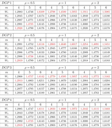
The data-generating processes (DGP s) studied are the following
DGP1 :Y =ρW X+ν X =ε DGP2 :Y = 1/(ρW X+ν) X =ε DGP3 :Y = (ρW X+ν)5 X =ε DGP4 :Y =sin(ρW X+ν) X =ε
whereεand v are normal standard distributed.
matricesW1,W2,W3,W4 andW5, each of them generated over an irregular (random) lattice. We estimate h(W X|Y) for sample size R = 400, three values of ρ = 0.5,1 and 2 and three values of m, namely, m= 4 (thus only 16 symbols are used to obtain a conclusion about the spatial structure of the spatial process Y),m= 5 (25 symbols are used) and m= 6 (36 symbols are used).
In the following table we present the results of the average value of theh(WiX|Y)
[image:10.595.106.491.258.695.2]for each i = 1,2,3,4 and 5 for a given model, with average computed over the total number of Monte Carlo replications.
Table 1: Simulations of Conditional Entropy
DGP1 ρ= 0.5 ρ= 1 ρ= 2
m 4 5 6 4 5 6 4 5 6
W1 1,2983 1,4746 1,6109 1,2798 1,4580 1,5955 1,1911 1,3723 1,5085 W2 1,2945 1,4767 1,6174 1,2946 1,4776 1,6163 1,2949 1,4772 1,6180
W3 1,2987 1,4771 1,6132 1,2966 1,4778 1,6120 1,2987 1,4774 1,6151
W4 1,2991 1,4735 1,6145 1,2998 1,4736 1,6141 1,3000 1,4742 1,6141 W5 1,2920 1,4790 1,6176 1,2904 1,4775 1,6175 1,2920 1,4773 1,6178
DGP2 ρ= 0.5 ρ= 1 ρ= 2
m 4 5 6 4 5 6 4 5 6
W1 1,2991 1,4752 1,6116 1,2863 1,4640 1,6017 1,2254 1,4091 1,5451 W2 1,2942 1,4765 1,6178 1,2945 1,4777 1,6166 1,2950 1,4774 1,6178
W3 1,2986 1,4776 1,6133 1,2968 1,4780 1,6121 1,2989 1,4775 1,6149
W4 1,2988 1,4736 1,6144 1,3001 1,4733 1,6140 1,2997 1,4736 1,6147 W5 1,2919 1,4789 1,6172 1,2904 1,4773 1,6181 1,2918 1,4776 1,6183
DGP3 ρ= 0.5 ρ= 1 ρ= 2
m 4 5 6 4 5 6 4 5 6
W1 1,2968 1,4757 1,6142 1,2779 1,4595 1,5957 1,1852 1,3772 1,5162 W2 1,2913 1,4863 1,6211 1,2904 1,4870 1,6202 1,2904 1,4863 1,6204 W3 1,2984 1,4792 1,6189 1,2993 1,4814 1,6190 1,2998 1,4784 1,6198
W4 1,2977 1,4795 1,6157 1,2981 1,4798 1,6154 1,2975 1,4785 1,6140
W5 1,2950 1,4761 1,6189 1,2961 1,4735 1,6197 1,2957 1,4763 1,6195
DGP4 ρ= 0.5 ρ= 1 ρ= 2
m 4 5 6 4 5 6 4 5 6
W1 1,2985 1,4747 1,6111 1,2833 1,4600 1,5972 1,2442 1,4115 1,5403 W2 1,2943 1,4769 1,6178 1,2945 1,4776 1,6162 1,2949 1,4769 1,6181
W3 1,2986 1,4772 1,6133 1,2966 1,4778 1,6121 1,2990 1,4776 1,6148
W4 1,2992 1,4735 1,6143 1,3000 1,4736 1,6139 1,3000 1,4744 1,6147 W5 1,2919 1,4791 1,6175 1,2903 1,4773 1,6176 1,2916 1,4778 1,6178
(correct) causal weighting matrix. Also, the detection of causal weighting matrix is more apparent as m increase. The last observation is also expected because, as m
grows, conditional entropy is evaluated on an increasing number of symbols and so a finer search is carried out.
To conclude this section we are going to simulate the following mixed data generating process:
[image:11.595.175.419.588.669.2]DGP5 :Y = 2ρW1X+ρW2X+ν X=ε
Table 2: Simulations of Conditional Entropy (DGP5)
ρ= 0.5 ρ= 1 ρ= 2
m 4 5 6 4 5 6 4 5 6
W1 1.2985 1,4747 1,6111 1,2833 1,4600 1,5972 1,2442 1,4115 1,5403 W2 1.2943 1,4769 1,6178 1,2945 1,4776 1,6162 1,2949 1,4769 1,6181 W3 1.2986 1,4772 1,6133 1,2966 1,4778 1,6121 1,2990 1,4776 1,6148
W4 1.2992 1,4735 1,6143 1,3000 1,4736 1,6139 1,3000 1,4744 1,6147 W5 1.2919 1,4791 1,6175 1,2903 1,4773 1,6176 1,2916 1,4778 1,6178
These results are very interesting because they stress the efficiency of the conditional entropy indicator to select the most relevant spatial structure. Data of variable Y have been obtained using two different weighting matrices, W1 and W2. The most important matrix isW1 because, inDGP5, the coefficient associated to this matrix is higher (doubles) than that associated to W2. As can be seen in the table above, the conditional entropy indicator, on average, always selects the W1 matrix (which is, indeed, the most influential) for high values of ρ and/or high values of m, the embedding dimension. Similar results are obtained with other combinations of weights.
5.2 The Causality Test
In continuation we present Monte Carlo results in relation to the performance of the ˆ
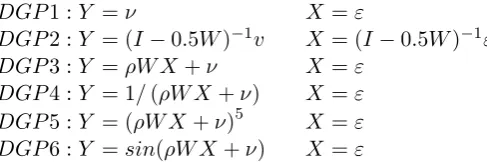
δ(W) statistic of (10) when applied to the problem of testing for causality in linear and nonlinear spatial processes. In order to conduct size and power experiments we have maintained the same collection of models of the previous section:
DGP1 :Y =ν X=ε DGP2 :Y = (I−0.5W)−1
v X= (I−0.5W)−1
ε DGP3 :Y =ρW X+ν X=ε
DGP4 :Y = 1/(ρW X+ν) X=ε DGP5 :Y = (ρW X+ν)5 X=ε DGP6 :Y =sin(ρW X+ν) X=ε
whereεand v are normal standard distributed and independent among them.
DGP′
s1−2 will be used to study the size of the test while DGP′
s3−6 will be used to study the power performance under linear and nonlinear processes.
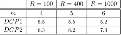
Table 3: Size performance of the ˆδ(W) statistic at 5% significance level
R= 100 R= 400 R= 1000
m 4 5 6
DGP1 5.5 5.5 5.2
DGP2 6.3 8.2 7.3
[image:12.595.138.457.282.385.2]a stable behavior around nominal levels for model 1, and values slightly higher but acceptable for model 2.
Table 4: Power performance of the ˆδ(W) statistic in porcentage
ρ= 0.5 ρ= 1 ρ= 2
m 4 5 6 4 5 6 4 5 6
R 100 400 1000 100 400 1000 100 400 1000
DGP3 6 10 13.5 20 39 85 73 99 100
DGP4 6 9.5 12 10 26.5 51.5 44 91 100
DGP5 6 10 12 22.5 39 69 74.5 99 100
DGP6 8 10.5 14 16 35 66 38.5 95.5 100
Table 4 reports the empirical power of the ˆδ(W) test on different sample sizes. As we can see, when ρ= 2, the power of our test against dependent processes is certainly satisfactory. For ρ= 1, the power of the test rapidly improves as the sample size and
m increases.
6
Conclusions
The purpose of this paper was twofold. In first place, we would like to claim for the importance of the question of causality also in a spatial context. This is one of the leading topics in mainstream Econometrics, surprisingly absent in the Spatial Econometrics agenda.
We contribute to this update with a nonparametric statistic that, specifically, tests for the existence of causality in a pair of variables. This test, which is not restricted to a spatial context, assesses the likelihood ‘arrow’ of causality between the two variables using a measure of conditional entropy and a bootstrapping. Furthermore, we complete the discussion with the development of a technique aimed at selecting the most influential spatial weighting matrix in a causal relation. According to our knowledge, there are few guidelines in relation to how choosing the spatial lag in a given model.
References
[1] Anselin, L. (1988). Spatial Econometrics: Methods and Models. Dordrecht, Kluwer.
[2] Anselin, L. and R. Florax (eds.) (1995).New Directions in Spatial Econometrics. Berlin, Springer.
[3] Anselin, L., Florax, R. and S. Rey (eds.) (2004). Advances in Spatial Econometrics: Methodology, Tools and Applications. Berlin, Springer.
[4] Ancona, N., D. Marinazzo and S. Stramaglia (2004): Radial Basis Function Approach to Nonlinear Granger Causality in Time Series, Physical Review E
70056221.
[5] Arbia, G. (2006).Spatial Econometrics. Statistical Foundations and Applications to Regional Convergence. Berlin, Springer.
[6] Diks, C. and V. Panchenko (2006): A New Statistic and Practical Guidelines for Nonparametric Granger Causality Testing. Journal of Economic Dynamics and Control 30, 1647-1669.
[7] Getis, A., Mur, J. and H. Zoller (eds.) (2004). Spatial Econometrics and Spatial Statistics. Houndmills, Macmillan.
[8] Griffith, D. (2003). Spatial Autocorrelation and Spatial Filtering: Gaining Understanding through Theory and Scientific Visualization. Berlin, Springer.
[9] Hong, Y. and H. White, H. (2005): Asymptotic Distribution Theory for Nonparametric Entropy Measures of Serial Dependence. Econometrica 73, 837-901.
[10] Joe, H. (1989a): Relative Entropy Measures of Multivariate Dependence.Journal of the American Statistical Association 84, 157-164.
[11] Joe, H. (1989b): Estimation of Entropy and Other Functionals of a Multivariate Density.Annals of the Institute of Statistical Mathematics 41, 683-697.
[12] Lesage, J. and Pace, K. (2009): Introduction to Spatial Econometrics. London, Chapman & Hall/CRC.
[14] Manrubia, S., A. Mikhailov and D. Zannette (2004): Emergence of Dynamical Order: Synchronization Phenomena in Complex Systems. Singapore: World Scientific Publishing.
[15] Marschinski, R. and H. Kantz (2002): Analysing the Information Flow between Financial Time Series- An Improved Estimator of Transfer Entropy. European Physical Journal B30, 275-281.
[16] Matilla-García, M. and M. Ruiz Marín (2008): A Non-Parametric Independence Test Using Permutation Entropy. Journal of Econometrics144, 139-155.
[17] Paelinck, J. and L. Klaassen (1979): Spatial Econometrics. Farnborough: Saxon House.
[18] Pearl, J. (2000). Causality: Models, Reasoning, and Inference. Cambridge: Cambridge University Press.
[19] Schreiber, T. (2000): Measuring Information Transfer. Physical Review Letters 85, 461-464.
[20] Suppes, P. (1970): A probabilistic Theory of Causality (Acta Philosophica Fennica. XXIV). Amsterdam: North-Holland.
[21] Tiefelsdorf, M. (2000): Modelling Spatial Processes. The Identification and Analysis of Spatial Relationships in Regression Residuals by Means of Moran’s I. Springer: Berlin.
[22] Upton, G. and B. Fingleton (1985): Spatial Data Analysis by Example, Vol. 1. New York, Wiley.