Mathematical Study of Dengue Disease Transmission in Multi Patch Environment

http://dx.doi.org/10.4236/am.2016.714132

Mathematical Study of Dengue Disease

Transmission in Multi-Patch Environment

Ganga Ram Phaijoo, Dil Bahadur Gurung

Department of Natural Sciences (Mathematics), School of Science, Kathmandu University, Dhulikhel, Nepal

Received 20 June 2016; accepted 21 August 2016; published 24 August 2016

Copyright © 2016 by authors and Scientific Research Publishing Inc.

This work is licensed under the Creative Commons Attribution International License (CC BY).

http://creativecommons.org/licenses/by/4.0/

Abstract

Dengue disease is the most common vector borne infectious disease transmitted to humans by in-fected adult female Aedes mosquitoes. Over the past several years the disease has been increasing remarkably and it has become a major public health concern. Dengue viruses have increased their geographic range into new human population due to travel of humans from one place to the other. In the present paper, we have proposed a multi patch SIR-SI model to study the host-vector dy-namics of dengue disease in different patches including the travel of human population among the patches. We have considered different disease prevalences in different patches and different

tra-vel rates of humans. The dimensionless number, basic reproduction number R0 which shows that

the disease dies out if R0 < 1 and the disease takes hold if R0≥ 1, is calculated. Local and global

sta-bility of the disease free equilibrium are analyzed. Simulations are observed considering the two patches only. The results show that controlling the travel of infectious hosts from high disease dominant patch to low disease dominant patch can help in controlling the disease in low disease dominant patch while high disease dominant becomes even more disease dominant. The under-standing of the effect of travel of humans on the spatial spread of the disease among the patches can be helpful in improving disease control and prevention measures. In the present study, a patch may represent a city, a village or some biological habitat.

Keywords

Dengue, Patch, Basic Reproduction Number, Equilibrium Point, Stability

1. Introduction

the person loses immunity to other serotype of viruses and becomes more susceptible in developing dengue he-morrhagic fever [1]. The prevalence of the disease has been increasing dramatically and the disease has become a major public health problem in recent years. According to World Health Organization, dengue has shown 30 fold increase globally over five decades. About 50 - 100 million new infections are estimated to occur annually in more than 100 endemic countries. Almost fifty percent of the world’s population lives in the countries where dengue is endemic [2].

There have been many mathematical studies to understand the dynamics of infectious diseases. Mathematical models can help in providing guides and suggestions for the control of the disease to the concerned authorities. Kermack and McKendrick introduced an SIR model to study the transmission of infectious diseases [3] which became very popular in the mathematical study of epidemic diseases. Esteva and Vargas proposed an SIR-SI model to study the transmission dynamics of dengue disease considering constant [4] and variable [5] host pop-ulations. Since then, different mathematical models have been proposed to study dengue disease transmission. Authors in [6] [7] studied the impact of awareness in the transmission of dengue disease. Pinho et al. [8] used mathematical model for dengue disease transmission with the aim of analyzing and comparing two dengue epi-demics that occurred in Brazil. Pongsumpun [9] studied the incubation period of dengue viruses using SEIR model. Edy and Supriatna proposed a two dimensional epidemic model to study the transmission of dengue dis-ease restricting the dynamics for two dimensions for the constant host and vector populations [10].

Emerging and re-emerging diseases like dengue disease spread very quickly due to the travel of infective hu-man population from one region to the other. They spread the disease in new regions. Different spatial models have been developed to study infectious diseases. Arino and Driessche [11] [12] studied the disease spread in meta-populations and they developed multicity model to study the infectious diseases in different cities. Wang and Mulone [13]; and Wang and Zhao [14] proposed epidemic models with population dispersal to describe the dynamics of disease spread between n patches and two patches. Hsieh et al. proposed a multi-patch epidemic model to study the impact travel between patches for the spatial spread of influenza [15].

Lee and Castillo-Chavez [16] formulated the two patch dengue transmission model to explore the role of res-idence times in dengue transmission dynamics and optimal control strategies assuming that only the human budgets their residence time across the patches. In the present work, we have discussed the multi-patch SIR-SI model to study the transmission dynamics of dengue disease among n-patches. We have investigated the impact of travel rates of humans in the transmission dynamics and control of dengue disease. We have assumed differ-ent travel rates and differdiffer-ent disease prevalences in differdiffer-ent patches.

2. Model Formulation

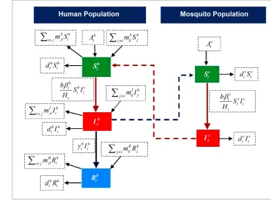
For the formulation of the model, we divide human population in three classes, susceptible, infective and recov-ered. Let Sih,

h i

I , Rih respectively denote the number of susceptible humans, infective humans and recovered humans in patch i. Also, we divide mosquito population in two compartments only, susceptible and infective mosquitoes. Let Siv,

v i

I respectively denote the number of susceptible mosquitoes and infective mosquitoes in patch i i

(

=1, 2, 3,,n

)

.

The SIR-SI Model for i=1, 2,,n for dengue disease transmission shown in Figure 1, whose parameters are discussed in Table 1, is described by the following system of differential equations

(

)

1 1 1 1 1 1 d d d d d d d d d d

h h n n

h h v h h S h S h

i i

i i i i i ij j ji i

j j

i

h h n n

h v h h h I h I h i i

i i i i i ij j ji i

j j

i

h n n

h h h h R h R h i

i i i i ij j ji i

j j

v v

v v h v v

i i

i i i i i i

v v i i

S b

A S I d S m S m S t H

I b

S I d I m I m I t H

R

I d R m R m R t

S b

A S I d S t H I b t H β β _γ γ β β = = = = = = = − − + − = − + + − = − + − = − − =

∑

∑

∑

∑

∑

∑

v h v v i i i i i

S I −d I

[image:3.595.104.497.85.378.2]

Figure 1. Flow chart of the model.

Table 1. Parameters used in the model.

Symbols Description

h i

d death rate in host population

v i

d death rate in vector population

h i

γ recovery rate of host population

h i

β transmission probability from vector to host

v i

β transmission probability from host to vector

b biting rate of vector

h i

A recruitment rate of host population

v i

A recruitment rate of vector population

, ,

S I R ij

m travel rate of susceptible, infective, recovered host population from patch j to patch i, i≠j where,

( )

( )

( )

( )

h h h

i i i i

S t +I t +R t =H t (Total host population in patch i in time t)

( )

( )

( )

v v

i i i

S t +I t =V t (Total vector population in patch i in time t) The total host and vector population sizes in all n-patches in time t is

( )

( )

( )

( )

1 1

,

n n

i i

i i

H t H t V t V t

= =

=

∑

=

∑

Theorem 1. The system of Equations (2.1) has a unique disease free equilibrium point.

In disease free situation,

1 1

0

n n

h h R h R h

i i ij j ji i

j j

d R m R m R

= =

− +

_∑

−

_∑

=

In matrix form,

0 h

R

ζ

− = (2.2) where,

1 1 12 1

1

21 2 2 2 T

2

1 2

1 2

, , , ,

h R R R

j n

j

R h R R

j n

h h h h

j

n

R R h R

n n n jn

j n

d m m m

m d m m

R R R R

m m d m

ζ ≠ ≠ ≠  + − −     _{− + −}    _{ } =_{ } =_{ }    _{− − +}     

∑

∑

∑

       

Here, ζ has all off-diagonal entries negative and every column has positive sum. So, ζ is a non-singular

M-matrix. Since all the off diagonal elements are non-zero, ζ is irreducible [17]. Hence, ζ has a positive in-verse and the system of Equations (2.2) has a unique solution. So, Rh =0 is the solution of the system, i.e.,

0 h i

R = for i=1, 2, 3,,n. Hence, in disease free situation, Iih=0, 0 v i

I = , Rih =0 for all i=1, 2, 3,,n. Also, h h*

i i

S =S , v v*

i i

S =S .

Now, we show that the disease free equilibrium is unique. From the system of Equations (2.1), in disease free situation:

For the host populations only:

1 1 12 1

* 1

1 1

*

21 2 2 2

2 2

2

*

1 2

h S S S

j n

h h

j

S h S S

h h

j n

j

h h

S S h S _{n n}

n n n jn

j n

d m m m

S A

m d m m _{S A}

S A

m m d m

≠ ≠ ≠  + − −   _{    }  _{− + −     }  _{    } =  _{    }  _{    }  _{− − +        }    

∑

∑

∑

         i.e., * h h

CS =A (2.3) where,

(

1

)

diag h n S S

i j ji

C= d +

∑

₌m −M ,

12 1 21 2 1 2 0 0 0 S S n S S S n S S n n m m m m M m m       =               

T _{* * * *} T

1, 2, , , 1 , 2 , ,

h h h h h h h h

n n

A =_A A  A _ S =_S S  S _

For vector populations only:

*

1 1 1

*

2 2 2

*

0 0

0 0

0 0

v v v

v v v

v v v

n n n

d S A

d S A

d S A

                 ₌                                  i.e., * v v

where,

( )

_{* * * *} T T

1 2 1 2

diag iv , v v, v , , nv , v v, v, , nv

D= d S =_S S  S _ A =_A A  A _

Here, the matrix C has positive column sums and each non-diagonal element is negative. So, the matrix C is an irreducible and non-singular M-matrix. Again, since C is an irreducible non-singular M-matrix, C must have posi-tive inverse, i.e., C−1>0 [17]. Hence, there is a unique solution Sh*=C A−1 h>0.

Also, the matrix D is a diagonal matrix with positive diagonal elements. So, there exists _D−1

with positive diagonal elements. Hence, Sv*=D A−1 v is unique solution of DSv*=Av. The results show that there always exists a unique disease free equilibrium point.

3. Basic Reproduction Number

Basic reproduction number R0 is defined as the expected number of secondary cases produced by a typical in-fective individual introduced into a completely susceptible population.

We use next generation matrix method [18] [19] to find the basic reproduction number. For, we order the in-fected variables by 1, 2, , , 1, 2, ,

h h h v v v

n n

I I  I I I  I . Then,

*

11 12

21 22 *

0 diag diag 0 h h i i i v v i i i b S H F F F

F F _b S H β β            =_{  }= _    _{  }    _{ }   

11 12 11

21 22 22

0 0

V V V V

V V V

    =_{  }= _     where,

( )

11 22 1

diag , diag

n

h h I I v

i i ji i

j

V d γ m M V d

=

 

= _ + + _− =



∑



Here, the matrix V11 has column sums, 1 0, , 0

h h

n

d >  d > and all off diagonal elements are negative. So, the matrix V11 is an irreducible non-negative M-matrix. Hence,

1 11

V− exists and is positive, i.e., V111 0 − _>

. Also, V22 is a diagonal matrix with positive entries. So, nonnegative

1 22

V− exists. The basic reproduction number R0 for the system (2.1) is the spectral radius of

{

}

1 1

FV− =ρ FV− . In fact,

1 _{1 1}

12 11 12

1 11 12 22

1 1

21 22 21 22 21 11

0 0 0 0 0

0 0 0 0 0

F V F V F V

FV

F V F V F V

− _{− −} − − −           =_{   } =_{   }= _          

Theorem 2. If R0 < 1, then the disease free equilibrium is locally asymptotically stable and unstable if R0 > 1.

Proof: Let J11 and J12 be the matrices of partial derivatives evaluated at the disease free equilibrium. The Jacobian matrix for the linearization of the system about the disease free equilibrium is obtained as the block structure 11 12 0 J J J F V   =  ₋   

Matrix J is triangular. So, the eigenvalues of J are those of the partition matrices J11 and F V− . Also,

11 0 0 C J D −   =  ₋   

Matrices C and D (matrices defined in Theorem 1) are non-singular M matrices. So, spectral abscissa,

( )

0,

( )

0

s −C < s −D < [17] and eigenvalues of the matrix J11 have negative real parts.

F V− will have negative real parts if and only if ρ

{

FV−1

}

<1 [19]. i.e., disease free equilibrium is locally asymptotically stable if and only if the basic reproduction number R0 ρ

{

FV 1

}

1

−

= < .

If R0>1, then s F

(

−V

)

>0. It shows that at least one eigenvalue lies in right half plane. So, the disease free equilibrium is unstable if R0>1.

Theorem 3. If R0 < 1, then the disease free equilibrium is globally asymptotically stable and unstable if R0 > 1.

Proof: Since, Sih ≤Sih* and

*

v v

i i

S ≤S , we have from the system of Equations (2.1),

(

)

* 1 1 * d d d d

h h n n

h v h h h I h I h i i

i i i i i ij j ji i

j j

i v v

v h v v i i

i i i i i

I b

S I d I m I m I t H

I b

S I d I t H β _γ β = = ≤ − + + − ≤ −

∑

∑

(3.1)

Consider the linear system

(

)

* 1 1 * d d d d

h h n n

h v h h h I h I h i i

i i i i i ij j ji i

j j

i v v

v h v v i i

i i i i i

I b

S I d I m I m I t H

I b

S I d I t H β _γ β = = = − + + − = −

∑

∑

(3.2)

The system of Equations (3.2) can be written as d dt =A

u

u (3.3) where, 1, 2, , , 1, 2, , T, .

h h h v v v

n n

I I I I I I A F V

 

=_{ } = −

u   Here, F is a non-negative matrix and V is a non-negative

M- matrix. So,

(

)

{

1

}

0 1

s F−V < ⇔ρ FV− <

i.e., Eigenvalues of F V− lie on left half plane if R0<1. Hence, each positive solution of (3.3) satisfies lim 0

t→∞u= (3.4)

i.e., lim ih 0, lim iv 0

t→∞I = t→∞I = for all i=1, 2, 3,, .n

Since all the variables in the system of Equations (2.1) are non-negative, the use of Comparison theorem [20] [21] leads to

lim h 0, lim v 0

i i

t→∞I = t→∞I = for all i=1, 2, 3,, .n (3.5)

From the system of Equations (2.1), we have

1 1

d d

h n n

h h R h R h i

i i ij j ji i

j j

R

d R m R m R

t = =

= − +

∑

−

∑

(3.6)

i.e., d , d

h

h

R

R

t = −ζ (In matrix form)

Here, ζ (matrix defined in Theorem 1) is non-singular M-matrix. So, all eigenvalues of −ζ lie in the left half plane. Hence,

lim ih 0, 1, 2, 3, ,

t→∞R = i=  n.

Again, as t→ ∞,

1 1

d d

d d

h n n

h h h S h S h

i

i i i ij j ji i

j j

v

v v v i

i i i

S

A d S m S m S

t

S

A d S

t = = = − + − = −

∑

∑

(3.7)

d d

h h h

S A CS

t   = − (3.8)

d d

v v v

S A DS

t  =  − (3.9)

Here, matrices C and D are non-singular M-matrices, all their eigenvalues lie in left half plane. Therefore, if Sh

and Sv be the homogeneous solutions of Equation (3.8) and Equation (3.9), then

lim_t→∞S_h=0 and lim_t→∞S_v =0

Matrix C is an irreducible, non-singular M-matrix. So, the matrix C has positive inverse. Sh* =C A−1 h is a par-ticular solution and Sh=Sh+Sh* is the general solution of Equation (3.8). Also, Matrix D is diagonal matrix with positive diagonal elements. So, D has an inverse with positive diagonal elements. Hence, Sv*=D A−1 v is a particular solution and Sv=Sv+Sv* is the general solution of Equation (3.9). And,

* *

limt→∞Sih=Sih, limt→∞Iih=0, limt→∞Rih=0, limt→∞Siv =Siv , limt→∞Iiv =0 for all i=1, 2, 3,, .n

Thus, as t→ ∞, we obtain the equilibrium point

(

Sih*, 0,, 0,Siv*, 0, 0,, 0

)

. Hence, the disease free equili-brium is globally asymptotically stable if R0<1. If R0>1 [19], Theorem 2 admits that the disease free equili-brium point is unstable.

4. For

n

= 2 (Considering Two Patches Only)

We have

* * * *

1 1 2 2 1 1 2 2

11 12 21 22

1 2 1 2

0, diag , , diag , , 0

h h h h v v v v

b S b S b S b S

F F F F

H H H H

β β β β

   

= = _{ } = _{ } =

   

and 1 1 21 12

11

21 2 2 12

h h I I

I h h I

d m m

V

m d m

γ

γ

 + + − 

=  _{− + +} 

 , 12 0, 21 0, 22 diag

(

1, 2

)

v v

V = V = V = d d

Basic Reproduction Number

{

₁

}

(

_{2 2}

)

₂

(

_{2 2}

)

2

(

)

_{2 2 2}1

0 01 02 02 01 01 02

1

2 2 4 1

2

R =ρ FV− = a R +R + _a R −R + a a− R R _

 

where,

(

)(

12 21

)

1 1 21 2 2 12 12 21

1

I I

h h I h h I I I

m m a

d m d m m m

γ γ

= +

+ + + + −

(

)

2 * *

1 1 1 1

01 ₂

1 1 1 1 21

h v h v

v h h I

b S S

R

d H d m

β β γ

=

+ + (Basic reproduction number, Patch 1)

(

)

2 * *

2 2 2 2

02 ₂

2 2 2 2 12

h v h v

v h h I

b S S

R

d H d m

β β γ

=

+ + (Basic reproduction number, Patch 2)

5. Numerical Results and Discussions

We considered the case of two patches and computed basic reproduction number R0 for the numerical results. The parameter values chosen for the simulation are: H1=579984, H2=420477 [22], 1 10000

v

A = , b=1 3,

1 0.75

h

β = [8], 1 0.75

v

β = , 2 1000

v

A = , 2 0.75

h

β = [8], 2 0.5

v

β = , 1 1 14 2

v v

d = =d [9], 1 0.00003914 2

h h

d = =d

[22], 1 1 14 2

h h

γ = =γ [9]. With 12 21 0, 01 1

I I

[image:7.595.85.470.355.605.2]

m =m = R > and R02<1. Thus, patch 1 is a high disease dominant patch and patch 2 is a low disease dominant patch.

dominant patch. So, the number of susceptible hosts in patch 2 increases initially due to the travel of susceptible hosts from patch 1. Afterwards, due to the interaction of susceptible hosts with infectious mosquitoes and due to the natural death of some humans, the susceptible host population starts decreasing.

When the susceptible hosts come in contact with infectious mosquitoes, hosts get infected. So, the population size of infected hosts increases (Figure 3). Eventually, the infected host population decreases to zero due to their recovery from the disease and due to the natural death of some humans.

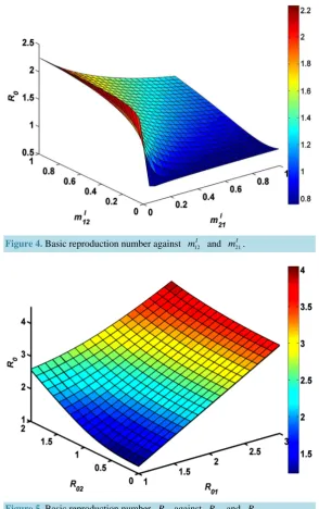
Changes in basic reproduction number R0 with the changes in travel rates are illustrated in Figure 4. It is observed that basic reproduction number R0 decreases with the increasing values of 21

I

m . Also, the number increases when the values of travel rate 12

I

[image:8.595.171.454.232.456.2]

m are increased. The figure shows that, the burden of disease reduces when the travel rates of hosts from high disease dominant patch to low disease dominant patch are high. The burden of disease increases when the travel rates of hosts from low disease dominant patch to the high disease

[image:8.595.169.456.473.709.2]

Figure 2.Dynamics of susceptible host population.

dominant patch are high. Thus, we should increase the travel rates of hosts from high disease dominant patch to the low disease dominant patch to bring the disease under control.

Basic reproduction number R0 of two patches is determined by the basic reproduction numbers, R01 of patch 1 and R02 of patch 2. Figure 5 shows that R0 increases together with R01 and R02. If basic repro-duction numbers of the both patches are high, then the basic reprorepro-duction number R0 gets higher. Thus, if any one of the two patches is more disease dominant and there is mobility between the two patches, then this can cause the whole system to be more endemic.

6. Discussion of Travel Restrictions

In this section, the dynamics of the host population is observed with the restriction of the travel of symptomatic hosts from one patch to the other patch.

[image:9.595.166.461.243.712.2]

Restricting the travel of symptomatic hosts from low disease dominant patch to high disease dominant patch

Figure 4.Basic reproduction number against ₁₂I

m and ₂₁I

[image:9.595.171.456.254.476.2]

m .

( 12 0

I

m = and keeping other parameters constant), Figure 6 shows that the burden of disease can be reduced in patch 1 but patch 2 becomes even more disease dominant (Figure 7).

Similarly, when 21 0

I

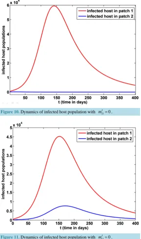
m = and all other parameters are same i.e., on restricting the travel of symptomatic trav-elers from high disease dominant patch to low disease dominant patch, we find that basic reproduction number of patch 1 increases (Figure 8) and basic reproduction number of patch 2 decreases (Figure 9). Thus, the dis-ease in low disdis-ease dominant patch can be controlled by restricting the travel of symptomatic hosts from high disease dominant patch to low disease dominant patch.

Dynamics of infected host populations are observed in Figure 10 and Figure 11 with travel restrictions. When infected hosts of patch 1 are restricted to travel (Figure 10) more hosts in patch 1 (very few hosts in patch 2) are observed infected of the disease when compared with the case that infected hosts of patch 2 are restricted (Figure 11) to travel. The graphical results (Figure 10, Figure 11) suggest that the disease spread in patch 2 can be brought under control by restricting the travel of infected hosts from patch 1 to patch 2.

Figure 6. Basic reproduction number of patch 1 against ₂₁I

m with ₁₂I 0

m = .

Figure 7.Basic reproduction number of patch 2 against ₂₁I

m with ₁₂I 0

[image:11.595.152.476.79.575.2]

Figure 8. Basic reproduction number of patch 1 against 12

I

m with 21 0

I

[image:11.595.158.469.85.323.2]

m = .

Figure 9. Basic reproduction number of patch 2 against ₁₂I

m with ₂₁I 0

m = .

7. Conclusions

In the present work, we have studied the effect of travel of humans on the transmission dynamics of dengue dis-ease. We discussed the disease transmission dynamics between n-patches by subdividing vector population in susceptible and infectious class and host population in susceptible, infectious and recovered class.

We defined the multi-patch basic reproduction number R0 by taking each patch together. Basic reproduction number R01 of patch 1 and R02 of patch 2 are calculated. The results show that the disease dies out if R0<1 and invades the population if R0>1. Theorem 2 and Theorem 3 show that the disease free equilibrium is lo-cally and globally asymptotilo-cally stable if R0<1 and unstable if R0>1.

[image:12.595.171.454.85.313.2]

Figure 10.Dynamics of infected host population with 21 0

I

m = .

Figure 11. Dynamics of infected host population with 12 0

I

m = .

dominant patch. Also, restricting the travel of infected hosts helps in controlling the disease. Basic reproduction number is seen higher when there is higher travel rate from low disease dominant patch to the high disease do-minant patch. The basic reproduction number is seen lowered when there is higher travel rate from high domi-nant disease patch to the low disease domidomi-nant patch. Thus, we can control the disease in low disease domidomi-nant patch by restricting the travel of infected hosts from high disease dominant patch.

References

[1] Gubler, D. (1998) Dengue and Dengue Hemorrhagic Fever. Clinical Microbiology Reviews, 3, 480-496.

[image:12.595.169.459.87.575.2]

[3] Kermack, W.O. and McKendrick, A.G. (1927) A Contribution to the Mathematical Theory of Epidemics. Proceedings of the Royal Society of London, 115, 700-721. http://dx.doi.org/10.1098/rspa.1927.0118

[4] Esteva, L. and Vargas, C. (1998) Analysis of a Dengue Disease Transmission Model. Mathematical Biosciences, 150, 131-151. http://dx.doi.org/10.1016/S0025-5564(98)10003-2

[5] Esteva, L. and Vargas, C. (1999) A Model for Dengue Disease with Variable Human Population. Journal of Mathe-matical Biology, 38, 220-240. http://dx.doi.org/10.1007/s002850050147

[6] Gakkhar, S. and Chavda, N.C. (2013) Impact of Awareness on the Spread of Dengue Infection in Human Population.

Applied Mathematics, 4, 142-147. http://dx.doi.org/10.4236/am.2013.48A020

[7] Phaijoo, G.R. and Gurung, D.B. (2015) Mathematical Study of Dengue Disease with and without Awareness in Host Population. International Journal of Advanced Engineering Research and Applications (IJAERA), 1, 239-245.

[8] Pinho, S.T.R., Ferreira, C.P., Esteva, L., Barreto, F.R., Morato e Silva, V.C. and Teixeira, M.G.L. (2010) Modelling the Dynamics of Dengue Real Epidemics. Philosophical Transactions of the Royal Society A, 368, 5679-5693. http://dx.doi.org/10.1098/rsta.2010.0278

[9] Pongsumpun, P. (2008) Mathematical Model of Dengue Disease with the Incubation Period of Virus. World Academy of Science, Engineering and Technology, 44, 328-332.

[10] Soewono, E. and Supriatna, A.K. (2001) A Two-Dimensional Model for the Transmission of Dengue Fever Disease.

Bulletin of the Malaysian Mathematical Sciences Society, 24, 49-57.

[11] Arino, J. and Van den Driessche, P. (2006) Disease Spread in Metapopulations. Field Institute Communications, 48, 1- 12.

[12] Arino, J. and van den Driessche, P. (2003) A Multicity Epidemic Model. Mathematical Population Studies, 10, 175- 193. http://dx.doi.org/10.1080/08898480306720

[13] Wang, W. and Mulone, G. (2003) Threshold of Disease Transmission in a Patch Environment. Journal of Mathemati-cal Analysis and Applications, 285, 321-335. http://dx.doi.org/10.1016/S0022-247X(03)00428-1

[14] Wang, W. and Zhao, X.Q. (2007) An Epidemic Model in a Patchy Environment. Mathematical Biosciences, 112, 97- 112.

[15] Hsieh, Y.H., van den Driessche, P. and Wang, L. (2007) Impact of Travel between Patches for Spatial Spread of Dis-ease. Bulletin of Mathematical Biology, 69, 1355-1375. http://dx.doi.org/10.1007/s11538-006-9169-6

[16] Lee, S. and Castillo-Chavez, C. (2015) The Role of Residence Times in Two-Patch Dengue Transmission Dynamics and Optimal Strategies. Journal of Theoretical Biology, 374, 152-164. http://dx.doi.org/10.1016/j.jtbi.2015.03.005 [17] Berman, A. and Plemmons, R.J. (1979) Non-Negative Matrices in Mathematical Sciences. Academic Press, New York.

[18] Diekmann, O., Heesterbeek, J.A.P. and Metz, J.A.J. (1990) On the Definition and Computation of the Basic Reproduc-tion Ratio RO in Models for Infectious Diseases in Heterogeneous Populations. Journal of Mathematical Biology, 28,

365-382. http://dx.doi.org/10.1007/BF00178324

[19] van den Driessche, P. and Watmough, J. (2007) Reproduction Numbers and Sub-Threshold Endemic Equilibria for Compartmental Models of Disease Transmission. Mathematical Biosciences, 180, 29-48.

http://dx.doi.org/10.1016/S0025-5564(02)00108-6

[20] Lakshmikantham, V., Leela, S. and Martynyuk, A.A. (1998) Stability Analysis of Non-Linear Systems. Dekker, Flori-da.

[21] Smith, H.L. and Waltman, P. (1995) The Theory of Chemostat. Cambridge University Press, New York. http://dx.doi.org/10.1017/CBO9780511530043

Submit or recommend next manuscript to SCIRP and we will provide best service for you:

Accepting pre-submission inquiries through Email, Facebook, LinkedIn, Twitter, etc. A wide selection of journals (inclusive of 9 subjects, more than 200 journals) Providing 24-hour high-quality service

User-friendly online submission system Fair and swift peer-review system

Efficient typesetting and proofreading procedure

Display of the result of downloads and visits, as well as the number of cited articles Maximum dissemination of your research work