A Survey of Cross-lingual Word Embedding Models
Sebastian Ruder [email protected]
Insight Research Centre, National University of Ireland, Galway, Ireland
Aylien Ltd., Dublin, Ireland
Ivan Vulić [email protected]
Language Technology Lab, University of Cambridge, UK
Anders Søgaard [email protected]
University of Copenhagen, Copenhagen, Denmark
Abstract
Cross-lingual representations of words enable us to reason about word meaning in multilingual contexts and are a key facilitator of cross-lingual transfer when developing natural language processing models for low-resource languages. In this survey, we provide a comprehensive typology of cross-lingual word embedding models. We compare their data requirements and objective functions. The recurring theme of the survey is that many of the models presented in the literature optimize for the same objectives, and that seemingly different models are often equivalent,modulo optimization strategies, hyper-parameters, and such. We also discuss the different ways cross-lingual word embeddings are evaluated, as well as future challenges and research horizons.
1. Introduction
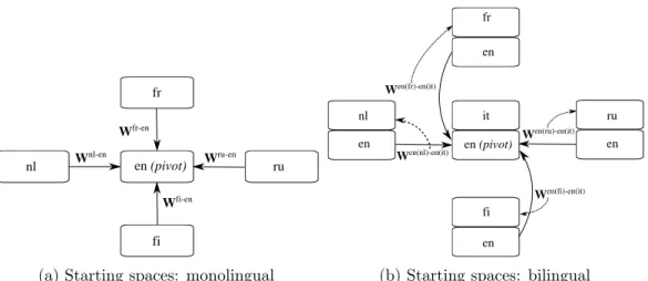
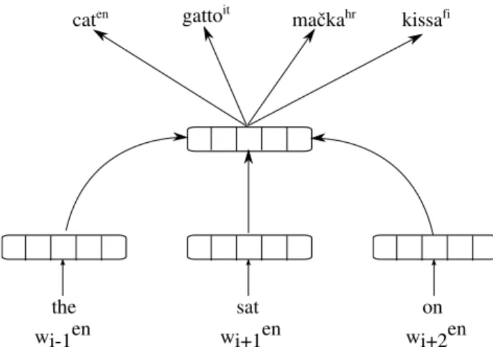
In recent years, (monolingual) vector representations of words, so-called word embeddings (Mikolov, Chen, Corrado, & Dean, 2013a; Pennington, Socher, & Manning, 2014) have proven extremely useful across a wide range of natural language processing (NLP) applications. In parallel, the public awareness of the digital language divide1, as well as the availability of multilingual benchmarks (Nivre et al., 2016a; Hovy, Marcus, Palmer, Ramshaw, & Weischedel, 2006; Sylak-Glassman, Kirov, Yarowsky, & Que, 2015), has made cross-lingual transfer a popular NLP research topic. The need to transfer lexical knowledge across languages has given rise tocross-lingual word embedding models, i.e., cross-lingual representations of words in a joint embedding space, as illustrated in Figure 1.
Cross-lingual word embeddings are appealing for two reasons: First, they enable us to compare the meaning of words across languages, which is key to bilingual lexicon induction, machine translation, or cross-lingual information retrieval, for example. Second, cross-lingual word embeddings enable model transfer between languages, e.g., between resource-rich and low-resource languages, by providing a common representation space. This duality is also reflected in how cross-lingual word embeddings are evaluated, as discussed in Section 10.
Many models for learning cross-lingual embeddings have been proposed in recent years. In this survey, we will give a comprehensive overview of existing cross-lingual word embedding models. One of the main goals of this survey is to show the similarities and differences between
1. E.g.,http://labs.theguardian.com/digital-language-divide/
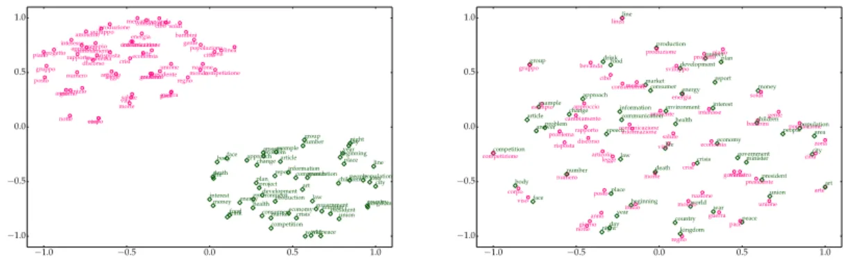
−1.0 −0.5 0.0 0.5 1.0 −1.0 −0.5 0.0 0.5 1.0 morte life city giorno rapporto example project bambini report piano competition union zona consumatore arte risposta mondo viso unione law vita informazione cibo body money approach market plan government consumer beginning corpo presidente ministro regno face world country numero esempio group death sviluppo health articolo gruppo governo answer line day guerra salute progetto economy area soldi bevanda ambiente crisi production people posto cambiamento popolazione energia year competizione mercato war problem anno interest minister linea kingdom information produzione legge approccio environment population number change problema nazione children gente president notte food energy art discorso inizio night communication peace citta development interesse crisis drink pace place article economia speech comunicazione −1.0 −0.5 0.0 0.5 1.0 −1.0 −0.5 0.0 0.5 1.0 morte life city giorno rapporto example project bambini report piano competition union zona consumatore arte risposta mondo viso unione law vita informazione cibo body money approach market plan government consumer beginning corpo presidente ministro regno face world country numero esempio group death sviluppo health articolo gruppo governo answer line day guerra salute progetto economy area soldi bevanda ambiente crisi production people posto cambiamento popolazione energia year competizione mercato war problem anno interest minister linea kingdom information produzione legge approccio environment population number change problema nazione childrengente president notte food energy art discorso inizio night communication peace citta development interesse crisis drink pace place article economia speechcomunicazione
Figure 1: Unaligned monolingual word embeddings (left) and word embeddings projected into a joint cross-lingual embedding space (right). Embeddings are visualized with t-SNE.
these approaches. To facilitate this, we first introduce a common notation and terminology in Section 2. Over the course of the survey, we then show that existing cross-lingual word embedding models can be seen as optimizing very similar objectives, where the main source of variation is due to the data used, the monolingual and regularization objectives employed, and how these are optimized. As many cross-lingual word embedding models are inspired by monolingual models, we introduce the most commonly used monolingual embedding models in Section 3. We then motivate and introduce one of the main contributions of this survey, a typology of cross-lingual embedding models in Section 4. The typology is based on the main differentiating aspect of cross-lingual embedding models: the nature of the data they require, in particular the type of alignment across languages (alignment of words, sentences, or documents), and whether data is assumed to be parallel or just comparable (about the same topic). The typology allows us to outline similarities and differences more concisely, but also starkly contrasts focal points of research with fruitful directions that have so far gone mostly unexplored.
Since the idea of cross-lingual representations of words pre-dates word embeddings, we provide a brief history of cross-lingual word representations in Section 5. Subsequent sections are dedicated to each type of alignment. We discuss cross-lingual word embedding algorithms that rely on word-level alignments in Section 6. Such methods can be further divided into mapping-based approaches, approaches based on pseudo-bilingual corpora, and joint methods. We show that these approaches, modulo optimization strategies and hyper-parameters, are nevertheless often equivalent. We then discuss approaches that rely on sentence-level alignments in Section 7, and models that require document-level alignments in Section 8. In Section 9, we describe how many bilingual approaches that deal with a pair of languages can be extended to the multilingual setting. We subsequently provide an extensive discussion of the tasks, benchmarks, and challenges of the evaluation of cross-lingual embedding models in Section 10 and outline applications in Section 11. We present general challenges and future research directions in learning cross-lingual word representations in Section 12. Finally, we provide our conclusions in Section 13.
This survey makes the following contributions:
1. It proposes a general typology that characterizes the differentiating features of cross-lingual word embedding models and provides a compact overview of these models.
2. It standardizes terminology and notation and shows that many cross-lingual word embedding models can be cast as optimizing nearly the same objective functions. 3. It provides a proof that connects the three types of word-level alignment models and
shows that these models are optimizing roughly the same objective.
4. It critically examines the standard ways of evaluating cross-lingual embedding models. 5. It describes multilingual extensions for the most common types of cross-lingual
embed-ding models.
6. It outlines outstanding challenges for learning cross-lingual word embeddings and provides suggestions for fruitful and unexplored research directions.
2. Notation and Terminology
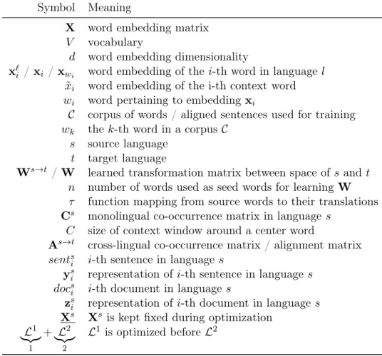
For clarity, we list all notation used throughout this survey in Table 1. We use bold lower case letters (x) to denote vectors, bold upper case letters (X) to denote matrices, and standard weight letters (x) for scalars. We use subscripts with bold letters (xi) to refer to entire rows or columns and subscripts with standard weight letters for specific elements (xi).
Let X`∈R|V
`|×d
be a word embedding matrix that is learned for the`-th ofL languages whereV`is the corresponding vocabulary anddis the dimensionality of the word embeddings. We will furthermore refer to the word embedding of the i-th word in language` with the shorthandx`i orxi if language`is clear from context. We will refer to the word corresponding to the i-th word embedding xi as wi where wi is a string. To make this correspondence clearer, we will in some settings slightly abuse index notation and use xwi to indicate the embedding corresponding to word wi. We will use ito index words based on their order in the vocabularyV, while we will use kto index words based on their order in a corpus C.
Some monolingual word embedding models use a separate embedding for words that occur in the context of other words. We will usex˜i as the embedding of thei-th context word and detail its meaning in the next section. Most approaches only deal with two languages, a source language sand a target language t.
Some approaches learn a matrixWs→tthat can be used to transform the word embedding matrixXsof the source languagesto that of the target languaget. We will designate such a matrix byWs→t∈
Rd×d andW if the language pairing is unambiguous. These approaches
often use nsource words and their translations as seed words. In addition, we will useτ as a function that maps from source words wis to their translationwti: τ :Vs→Vt. Approaches that learn a transformation matrix are usually referred to asoffline ormapping methods. As one of the goals of this survey is to standardize nomenclature, we will use the termmapping in the following to designate such approaches.
Some approaches require a monolingual word-word co-occurrence matrix Cs in language
s. In such a matrix, every row corresponds to a wordwsi and every column corresponds to a context wordwsj. Csij then captures the number of times wordwi occurs with context word
wj usually within a window of size C to the left and right of word wi. In a cross-lingual context, we obtain a matrix of alignment counts As→t ∈ R|V
t|×|Vs|
, where each element
Asij→t captures the number of times thei−th word in languaget was aligned with thej-th word in languages, with each row normalized to sum to1.
Symbol Meaning
X word embedding matrix
V vocabulary
d word embedding dimensionality
x`i /xi /xwi word embedding of thei-th word in languagel ˜
xi word embedding of the i-th context word
wi word pertaining to embeddingxi
C corpus of words / aligned sentences used for training
wk thek-th word in a corpus C
s source language
t target language
Ws→t /W learned transformation matrix between space ofsand t n number of words used as seed words for learning W
τ function mapping from source words to their translations
Cs monolingual co-occurrence matrix in languages C size of context window around a center word
As→t cross-lingual co-occurrence matrix / alignment matrix
sentsi i-th sentence in language s
ysi representation of i-th sentence in language s docs
i i-th document in language s
zsi representation of i-th document in languages
Xs Xs is kept fixed during optimization
L1 |{z} 1 + L2 |{z} 2 L1 is optimized beforeL2
Table 1: Notation used throughout this survey.
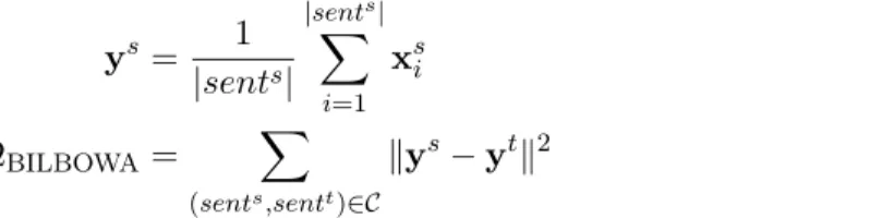
Finally, as some approaches rely on pairs of aligned sentences, we use sents1, . . . , sentsn to designate sentences in source languageswith representationsy1s, . . . ,ysn wherey∈Rd. We
analogously refer to their aligned sentences in the target language tas sentt1, . . . , senttn with representationsy1t, . . . ,ytn. We adopt an analogous notation for representations obtained by approaches based on alignments of documents in sandt: docs1, . . . , docsn anddoct1, . . . , doctn
with document representations zs1, . . . ,zsn and z1t, . . . ,ztn respectively where z∈Rd.
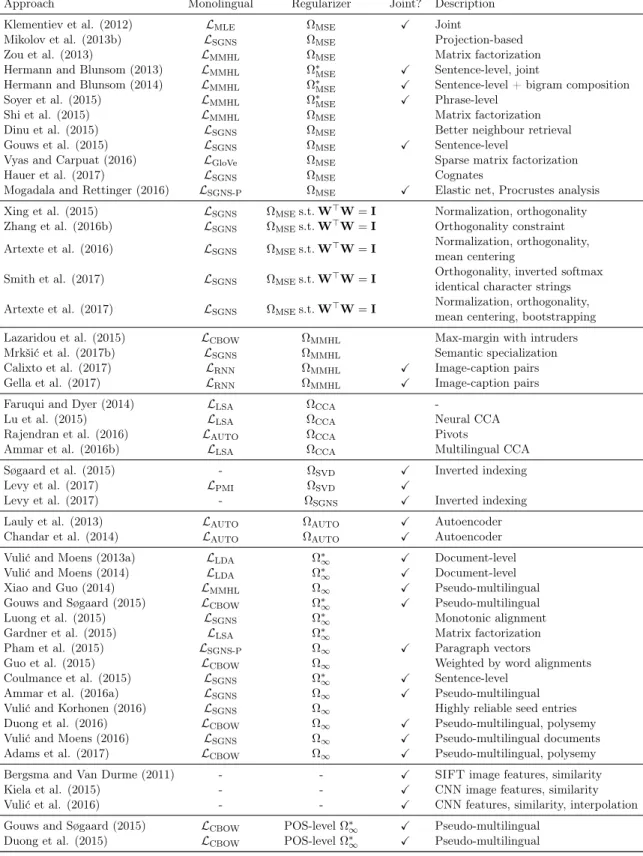
Different notations make similar approaches appear different. Using the same notation across our survey facilitates recognizing similarities between the various cross-lingual word embedding models. Specifically, we intend to demonstrate that cross-lingual word embedding models are trained by minimizing roughly the same objective functions, and that differences in objective are unlikely to explain the observed performance differences (Levy, Søgaard, & Goldberg, 2017).
The class of objective functions minimized by most cross-lingual word embedding methods (if not all), can be formulated as follows:
whereL`is the monolingual loss of thel-th language andΩis a regularization term. A similar loss was also defined by Upadhyay, Faruqui, Dyer, and Roth (2016). As recent work (Levy & Goldberg, 2014; Levy, Goldberg, & Dagan, 2015) shows that many monolingual losses are very similar, one of the main contributions of this survey is to condense the difference between approaches into a regularization term and to detail the assumptions that underlie different regularization terms.
Importantly, how this objective function is optimized is a key characteristic and differen-tiating factor between different approaches. The joint optimization of multiple non-convex losses is difficult. Most approaches thus take a step-wise approach and optimize one loss at a time while keeping certain variables fixed. Such a step-wise approach is approximate as it does not guarantee to reach even a local optimum.2 In most cases, we will use a longer formulation such as the one below in order to decompose in what order the losses are optimized and which variables they depend on:
J =L(Xs) +L(Xt) | {z } 1 + Ω(Xs,Xt,W) | {z } 2 (2)
The underbraces indicate that the two monolingual loss terms on the left, which depend onXs and Xt respectively, are optimized first. Note that this term decomposes into two separate monolingual optimization problems. Subsequently,Ω is optimized, which depends onXs,Xt,W. Underlined variables are kept fixed during optimization of the corresponding loss.
The monolingual losses are optimized by training one of several monolingual embedding models on a monolingual corpus. These models are outlined in the next section.
3. Monolingual Embedding Models
The majority of cross-lingual embedding models take inspiration from and extend monolingual word embedding models to bilingual settings, or explicitly leverage monolingually trained models. As an important preliminary, we thus briefly review monolingual embedding models that have been used in the cross-lingual embeddings literature.
Latent Semantic Analysis (LSA) Latent Semantic Analysis (Deerwester, Dumais, Fur-nas, Landauer, & Harshman, 1990) has been one of the most widely used methods for learning dense word representations. LSA is typically applied to factorize a sparse word-word co-occurrence matrix C obtained from a corpus. A common preprocessing method is to replace every entry in Cwith its pointwise mutual information (PMI) (Church & Hanks, 1990) score: P M I(wi, wj) = log p(wi, wj) p(wi)p(wj) = log#(wi, wj)· |C| #(wi)·#(wj) (3) where#(·) counts the number of (co-)occurrences in the corpusC. As for unobserved word pairs, P M I(wi, wj) = log 0 =∞, such values are often set to P M I(wi, wj) = 0, which is also known as positive PMI.
2. Other strategies such as alternating optimization methods, e.g. EM (Dempster, Laird, & Rubin, 1977) could be used with the same objective.
The PMI matrix P where Pi,j =P M I(wi, wj) is then factorized using singular value decomposition (SVD), which decomposesP into the product of three matrices:
P=UΨV> (4)
whereUandVare in column orthonormal form andΨis a diagonal matrix of singular values. We subsequently obtain the word embedding matrix Xby reducing the word representations to dimensionalityk the following way:
X=UkΨk (5)
where Ψk is the diagonal matrix containing the topksingular values and Uk is obtained by selecting the corresponding columns fromU.
Max-margin loss (MML) Collobert and Weston (2008) learn word embeddings by training a model on a corpusC to output a higher score for a correct word sequence than for an incorrect one. For this purpose, they use a max-margin or hinge loss3:
LMML = |C|−C X k=C+1 X w0∈V max(0,1−f([xwk−C, . . . ,xwi, . . . ,xwk+C]) +f([xwk−C, . . . ,xw0, . . . ,xwk+C])) (6)
The outer sum iterates over all words in the corpusC, while the inner sum iterates over all words in the vocabulary. Each word sequence consists of a center word wk and a window of C words to its left and right. The neural network, which is given by the functionf(·), consumes the sequence of word embeddings corresponding to the window of words and outputs a scalar. Using this max-margin loss, it is trained to produce a higher score for a word window occurring in the corpus (the top term) than a word sequence where the center word is replaced by an arbitrary word w0 from the vocabulary (the bottom term).
Skip-gram with negative sampling (SGNS) Skip-gram with negative sampling (Mikolov et al., 2013a) is arguably the most popular method to learn monolingual word embeddings due to its training efficiency and robustness (Levy et al., 2015). SGNS approximates a language model but focuses on learning efficient word representations rather than accurately modeling word probabilities. It induces representations that are good at predicting surrounding context words given a target word wk. To this end, it minimizes the negative log-likelihood of the training data under the followingskip-gram objective:
LSGNS=− 1 |C| −C |C|−C X k=C+1 X −C≤j≤C,j6=0 logP(wk+j|wk) (7)
P(wk+j|wk) is computed using the softmax function:
P(wk+j|wk) = exp(˜xwk+j >x wk) P|V| i=1exp(˜xwi >x wk) (8)
3. Equations in the literature slightly differ in how they handle corpus boundaries. To make comparing between different monolingual methods easier, we define the sum as starting with the(C+ 1)-th word in the corpusC (so that the first window includes the first wordw1) and ending with the(|C| −C)-th word
where xi andx˜i are the word and context word embeddings of wordwi respectively. The skip-gram architecture can be seen as a simple neural network: The network takes as input a one-hot representation of a word∈R|V| and produces a probability distribution over the vocabulary ∈ R|V|. The embedding matrix X and the context embedding matrix X˜ are simply the input-hidden and (transposed) hidden-output weight matrices respectively. The neural network has no nonlinearity, so is equivalent to a matrix product (similar to Equation 4) followed by softmax.
As the partition function in the denominator of the softmax is expensive to compute, SGNS uses Negative Sampling, which approximates the softmax to make it computationally more efficient. Negative sampling is a simplification of Noise Contrastive Estimation (Gutmann & Hyvärinen, 2012), which was applied to language modeling by Mnih and Teh (2012). Similar to noise contrastive estimation, negative sampling trains the model to distinguish a target word wk from negative samples drawn from a ‘noise distribution’Pn. In this regard, it is similar to MML as defined above, which ranks true sentences above noisy sentences. Negative sampling is defined as follows:
P(wk+j|wk) = logσ(x˜wk+j >x wk) + N X i=1 Ewi∼Pnlogσ(−x˜wi >x wk) (9)
whereσ is the sigmoid functionσ(x) = 1/(1 +e−x)andN is the number of negative samples. The distribution Pn is empirically set to the unigram distribution raised to the 3/4th power. Levy and Goldberg (2014) observe that negative sampling does not in fact minimize the negative log-likelihood of the training data as in Equation 7, but rather implicitly factorizes a shifted PMI matrix similar to LSA.
Continuous bag-of-words (CBOW) While skip-gram predicts each context word sepa-rately from the center word, continuous bag-of-words jointly predicts the center word based on all context words. The model receives as input a window ofC context words and seeks to predict the target wordwk by minimizing the CBOW objective:
LCBOW=− 1 |C| −C |C|−C X k=C+1 logP(wk|wk−C, . . . , wk−1, wk+1, . . . , wk+C) (10) P(wk|wk−C, . . . , wk+C) = exp(˜xwk >x¯ wk) P|V| i=1exp(˜xwi >¯x wk) (11) where x¯wk is the sum of the word embeddings of the words wk−C, . . . , wk+C, i.e. ¯xwk = P
−C≤j≤C,j6=0xwk+j. The CBOW architecture is typically also trained with negative sampling for the same reason as the skip-gram model.
Global vectors (GloVe) Global vectors (Pennington et al., 2014) allows us to learn word representations via matrix factorization. GloVe minimizes the difference between the dot product of the embeddings of a word xwi and its context word ˜xwj and the logarithm of their number of co-occurrences within a certain window size4:
4. GloVe favors slightly larger window sizes (up to 10 words to the right and to the left of the target word) compared to SGNS (Levy et al., 2015).
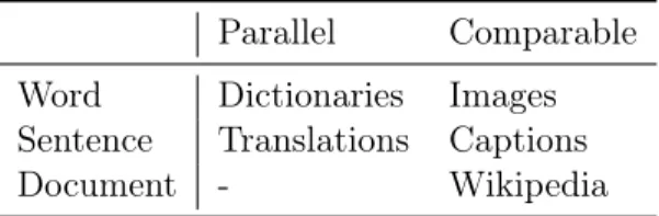
Parallel Comparable
Word Dictionaries Images
Sentence Translations Captions
Document - Wikipedia
Table 2: Nature and alignment level of bilingual data sources required by cross-lingual embedding models. LGloVe= |V| X i,j=1 f(Cij)(xwi > ˜ xwj+bi+ ˜bj −logCij) 2 (12)
where bi and ˜bj are the biases corresponding to word wi and word wj, Cij captures the number of times word wi occurs with wordwj, andf(·) is a weighting function that assigns relatively lower weight to rare and frequent co-occurrences. If we fix bi = log #(wi) and ˜bj = log #(wj), then GloVe is equivalent to factorizing a PMI matrix, shifted bylog|C|(Levy et al., 2015).
4. Cross-Lingual Word Embedding Models: Typology
Recent work on cross-lingual embedding models suggests that the actual choice of bilingual supervision signal—that is, the data a method requires to learn to align a cross-lingual representation space—is more important for the final model performance than the actual underlying architecture (Upadhyay et al., 2016; Levy et al., 2017). In other words, large differences between models typically stem from their data requirements, while other fine-grained differences are artifacts of the chosen architecture, hyper-parameters, and additional tricks and fine-tuning employed. This directly mirrors the argument raised by Levy et al. (2015) regarding monolingual embedding models: They observe that the architecture is less
important as long as the models are trained under identical conditions on the same type (and amount) of data.
We therefore base our typology on the data requirements of the cross-lingual word embedding methods, as this accounts for much of the variation in performance. In particular, methods differ with regard to the data they employ along the following two dimensions:
1. Type of alignment: Methods use different types of bilingual supervision signals (at the level of words, sentences, or documents), which introduce stronger or weaker
supervision.
2. Comparability: Methods require either parallel data sources, that is, exact transla-tions in different languages orcomparable data that is only similar in some way. In particular, there are three different types of alignments that are possible, which are required by different methods. We discuss the typical data sources for both parallel and comparable data based on the following alignment signals:
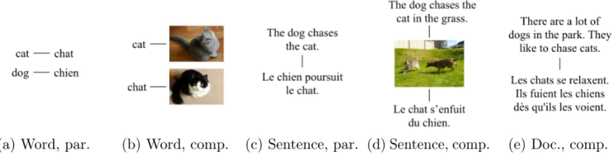
(a) Word, par. (b) Word, comp. (c) Sentence, par. (d) Sentence, comp. (e) Doc., comp. Figure 2: Examples for the nature and type of alignment of data sources. Par.: parallel. Comp.: comparable. Doc.: document. From left to right, word-level parallel alignment in the form of a bilingual lexicon (2a), word-level comparable alignment using images obtained with Google search queries (2b), sentence-level parallel alignment with translations (2c), sentence-level comparable alignment using translations of several image captions (2d), and document-level comparable alignment using similar documents (2e).
1. Word alignment: Most approaches use parallel word-aligned data in the form of bilingual or cross-lingual dictionary with pairs of translations between words in different languages (Mikolov, Le, & Sutskever, 2013b; Faruqui & Dyer, 2014b). Parallel word alignment can also be obtained by automatically aligning words in a parallel corpus (see below), which can be used to produce bilingual dictionaries. Throughout this survey, we thus do not differentiate between the source of word alignment, whether it comes from type-aligned (dictionaries) or token-aligned data (automatically aligned parallel corpora). Comparable word-aligned data, even though more plentiful, has been leveraged less often and typically involves other modalities such as images (Bergsma & Van Durme, 2011; Kiela, Vulić, & Clark, 2015).
2. Sentence alignment: Sentence alignment requires a parallel corpus, as commonly used in machine translation (MT). Methods typically use the Europarl corpus (Koehn, 2005), which consists of sentence-aligned text from the proceedings of the European parliament, and is perhaps the most common source of training data for MT models (Hermann & Blunsom, 2013; Lauly, Boulanger, & Larochelle, 2013). Other methods use available word-level alignment information (Zou, Socher, Cer, & Manning, 2013; Shi, Liu, Liu, & Sun, 2015). There has been some work on extracting parallel data from comparable corpora (Munteanu & Marcu, 2006), but no-one has so far trained cross-lingual word embeddings on such data. Comparable data with sentence alignment may again leverage another modality, such as captions of the same image or similar images in different languages, which are not translations of each other (Calixto, Liu, & Campbell, 2017; Gella, Sennrich, Keller, & Lapata, 2017).
3. Document alignment: Parallel document-aligned data requires documents in differ-ent languages that are translations of each other. This is rare, as parallel documdiffer-ents typically consist of aligned sentences (Hermann & Blunsom, 2014). Comparable document-aligned data is more common and can occur in the form of documents that are topic-aligned (e.g. Wikipedia) or class-aligned (e.g. sentiment analysis and
multi-class classification datasets) (Vulić & Moens, 2013b; Mogadala & Rettinger, 2016).
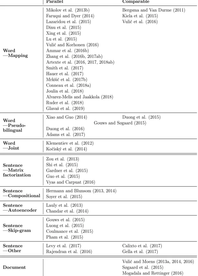
We summarize the different types of data required by cross-lingual embedding models along these two dimensions in Table 2 and provide examples for each in Figure 2. Over the course of this survey we will show that models that use a particular type of data are mostly variations of the same or similar architectures. We present our complete typology of cross-lingual embedding models in Table 3, aiming to provide an exhaustive overview by classifying each model (we are aware of) into one of the corresponding model types. We also provide a more detailed overview of the monolingual objectives and regularization terms used by every approach towards the end of this survey in Table 5.
5. A Brief History of Cross-Lingual Word Representations
We provide a brief overview of the historical lineage of cross-lingual word embedding models. In brief, while cross-lingual word embeddings is a novel phenomenon, many of the high-level ideas that motivate current research in this area, can be found in work that pre-dates the popular introduction of word embeddings. This includes work on learning cross-lingual word representations from seed lexica, parallel data, or document-aligned data, as well as ideas on learning from limited bilingual supervision.
Language-independent representations have been proposed for decades, many of which rely on abstract linguistic labels instead of lexical features (Aone & McKee, 1993; Schultz & Waibel, 2001). This is also the strategy used in early work on so-called delexicalized cross-lingual and domain transfer (Zeman & Resnik, 2008; Søgaard, 2011; McDonald, Petrov, & Hall, 2011; Cohen, Das, & Smith, 2011; Täckström, McDonald, & Uszkoreit, 2012; Henderson, Thomson, & Young, 2014), as well as in work on inducing cross-lingual word clusters (Täckström et al., 2012; Faruqui & Dyer, 2013), and cross-lingual word embeddings relying on syntactic/POS contexts (Duong, Cohn, Bird, & Cook, 2015; Dehouck & Denis, 2017).5 The ability to represent lexical items from two different languages in a shared cross-lingual space supplements seminal work in cross-cross-lingual transfer by providing fine-grained word-level links between languages; see work in cross-lingual dependency parsing (Ammar, Mulcaire, Ballesteros, Dyer, & Smith, 2016a; Zeman et al., 2017) and natural language understanding systems (Mrkšić et al., 2017b).
Similar to our typology of cross-lingual word embedding models outlined in Table 3 based on bilingual data requirements from Table 2, one can also arrange older cross-lingual representation architectures into similar categories. A traditional approach to cross-lingual vector space induction was based on high-dimensional context-counting vectors where each dimension encodes the (weighted) co-occurrences with a specific context word in each of the languages. The vectors are then mapped into a single cross-lingual space using a seed bilingual dictionary containing paired context words from both sides (Rapp, 1999; Gaussier, Renders, Matveeva, Goutte, & Déjean, 2004; Laroche & Langlais, 2010; Tamura, Watanabe, & Sumita, 2012, inter alia). This approach is an important predecessor to the cross-lingual
5. Along the same line, the recent initiative on providing cross-linguistically consistent sets of such labels (e.g., Universal Dependencies, Nivre et al., 2016) facilitates cross-lingual transfer and offers further support to the induction of word embeddings across languages (Vulić, 2017; Vulić, Schwartz, Rappoport, Reichart, & Korhonen, 2017).
Parallel Comparable
Word —Mapping
Mikolov et al. (2013b) Bergsma and Van Durme (2011) Faruqui and Dyer (2014) Kiela et al. (2015)
Lazaridou et al. (2015) Vulić et al. (2016) Dinu et al. (2015)
Xing et al. (2015) Lu et al. (2015)
Vulić and Korhonen (2016) Ammar et al. (2016b) Zhang et al. (2016b, 2017ab) Artexte et al. (2016, 2017, 2018ab) Smith et al. (2017)
Hauer et al. (2017) Mrkšić et al. (2017b) Conneau et al. (2018a) Joulin et al. (2018)
Alvarez-Melis and Jaakkola (2018) Ruder et al. (2018)
Glavaš et al. (2019)
Word —Pseudo-bilingual
Xiao and Guo (2014) Duong et al. (2015) Gouws and Søgaard (2015) Duong et al. (2016) Adams et al. (2017) Word —Joint Klementiev et al. (2012) Kočiský et al. (2014) Sentence —Matrix factorization Zou et al. (2013) Shi et al. (2015) Gardner et al. (2015) Guo et al. (2015) Vyas and Carpuat (2016)
Sentence
—Compositional
Hermann and Blunsom (2013, 2014) Soyer et al. (2015) Sentence —Autoencoder Lauly et al. (2013) Chandar et al. (2014) Sentence —Skip-gram Gouws et al. (2015) Luong et al. (2015) Coulmance et al. (2015) Pham et al. (2015) Sentence —Other
Levy et al. (2017) Calixto et al. (2017) Rajendran et al. (2016) Gella et al. (2017)
Document
Vulić and Moens (2013a, 2014, 2016) Søgaard et al. (2015)
Mogadala and Rettinger (2016)
word embedding models described in Section 6. Similarly, the bootstrapping technique developed for traditional context-counting approaches (Peirsman & Padó, 2010; Vulić & Moens, 2013b) is an important predecessor to recent iterative self-learning techniques used to limit the bilingual dictionary seed supervision needed in mapping-based approaches (Hauer, Nicolai, & Kondrak, 2017; Artetxe, Labaka, & Agirre, 2017). The idea of CCA-based word embedding learning (see later in Section 6; Faruqui & Dyer, 2014b; Lu, Wang, Bansal, Gimpel, & Livescu, 2015) was also introduced a decade earlier (Haghighi, Liang, Berg-Kirkpatrick, & Klein, 2008); their word additionally discussed the idea of combining orthographic subword features with distributional signatures for cross-lingual representation learning: This idea re-entered the literature recently (Heyman, Vulić, & Moens, 2017), only now with much better performance.
Cross-lingual word embeddings can also be directly linked to the work on word alignment for statistical machine translation (Brown, Pietra, Pietra, & Mercer, 1993; Och & Ney, 2003). Levy et al. (2017) stress that word translation probabilities extracted from sentence-aligned parallel data by IBM alignment models can also act as the cross-lingual semantic similarity function in lieu of the cosine similarity between word embeddings. Such word translation tables are then used to induce bilingual lexicons. For instance, aligning each word in a given source language sentence with the most similar target language word from the target language sentence is exactly the same greedy decoding algorithm that is implemented in IBM Model 1. Bilingual dictionaries and cross-lingual word clusters derived from word alignment links can be used to boost cross-lingual transfer for applications such as syntactic parsing (Täckström et al., 2012; Durrett, Pauls, & Klein, 2012), POS tagging (Agić, Hovy, & Søgaard, 2015), or semantic role labeling (Kozhevnikov & Titov, 2013) by relying on shared lexical information stored in the bilingual lexicon entries. Exactly the same functionality can be achieved by cross-lingual word embeddings. However, cross-lingual word embeddings have another advantage in the era of neural networks: the continuous representations can be plugged into current end-to-end neural architectures directly as sets of lexical features.
A large body of work on multilingual probabilistic topic modeling (Vulić, De Smet, Tang, & Moens, 2015; Boyd-Graber, Hu, & Mimno, 2017) also extracts shared cross-lingual word spaces, now by means of conditional latent topic probability distributions: two words with similar distributions over the induced latent variables/topics are considered semantically similar. The learning process is again steered by the data requirements. The early days witnessed the use of pseudo-bilingual corpora constructed by merging aligned document pairs, and then applying a monolingual representation model such as LSA (Landauer & Dumais, 1997) or LDA (Blei, Ng, & Jordan, 2003) on top of the merged data (Littman, Dumais, & Landauer, 1998; De Smet, Tang, & Moens, 2011). This approach is very similar to the pseudo-cross-lingual approaches discussed in Section 6 and Section 8. More recent topic models learn on the basis of parallel word-level information, enforcing word pairs from seed bilingual lexicons (again!) to obtain similar topic distributions (Boyd-Graber & Blei, 2009; Zhang, Mei, & Zhai, 2010; Boyd-Graber & Resnik, 2010; Jagarlamudi & Daumé III, 2010). In consequence, this also influences topic distributions of related words not occurring in the dictionary. Another group of models utilizes alignments at the document level (Mimno, Wallach, Naradowsky, Smith, & McCallum, 2009; Platt, Toutanova, & Yih, 2010; Vulić, De Smet, & Moens, 2011; Fukumasu, Eguchi, & Xing, 2012; Heyman, Vulić, & Moens, 2016) to induce shared topical spaces. The very same level of supervision (i.e., document
alignments) is used by several cross-lingual word embedding models, surveyed in Section 8. Another embedding model based on the document-aligned Wikipedia structure (Søgaard, Agić, Alonso, Plank, Bohnet, & Johannsen, 2015) bears resemblance with the cross-lingual Explicit Semantic Analysis model (Gabrilovich & Markovitch, 2006; Hassan & Mihalcea, 2009; Sorg & Cimiano, 2012).
All these “historical” architectures measure the strength of cross-lingual word similarities through metrics defined in the cross-lingual space: e.g., Kullback-Leibler or Jensen-Shannon divergence (in a topic space), or vector inner products (in sparse context-counting vector space),and are therefore applicable to NLP tasks that rely cross-lingual similarity scores. The pre-embedding architectures and more recent cross-lingual word embedding methods have been applied to an overlapping set of evaluation tasks and applications, ranging from bilingual lexicon induction to cross-lingual knowledge transfer, including cross-lingual parser transfer (Täckström et al., 2012; Ammar et al., 2016a), cross-lingual document classification (Gabrilovich & Markovitch, 2006; De Smet et al., 2011; Klementiev, Titov, & Bhattarai, 2012; Hermann & Blunsom, 2014), cross-lingual relation extraction (Faruqui & Kumar, 2015), etc. In summary, while sharing the goals and assumptions of older cross-lingual architectures, cross-cross-lingual word embedding methods have capitalized on the recent methodological and algorithmic advances in the field of representation learning, owing their wide use to their simplicity, efficiency and handling of large corpora, as well as their relatively robust performance across domains.
6. Word-Level Alignment Models
In the following, we will now discuss different types of the current generation of cross-lingual embedding models, starting with models based on word-level alignment. Among these, models based on parallel data are more common.
6.1 Word-level Alignment Methods with Parallel Data We distinguish three methods that use parallel word-aligned data:
a) Mapping-based approachesthat first train monolingual word representations inde-pendently on large monolingual corpora and then seek to learn a transformation matrix that maps representations in one language to the representations of the other language. They learn this transformation from word alignments or bilingual dictionaries (we do not see a need to distinguish between the two).
b) Pseudo-multi-lingual corpora-based approachesthat use monolingual word em-bedding methods on automatically constructed (or corrupted) corpora that contain words from both the source and the target language.
c) Joint methodsthat take parallel text as input and minimize the source and target language monolingual losses jointly with the cross-lingual regularization term.
We will show thatmodulooptimization strategies, these approaches are equivalent. Before discussing the first category of methods, we briefly introduce two concepts that are of relevance in these and the subsequent sections.
Bilingual lexicon induction Bilingual lexicon induction is the intrinsic task that is most commonly used to evaluate current cross-lingual word embedding models. Briefly, given a list of N language word forms ws1, . . . , wsN, the goal is to determine the most appropriate translationwti, for each query formwis. This is commonly accomplished by finding a target language word whose embeddingxti is the nearest neighbour to the source word embedding
xsi in the shared semantic space, where similarity is usually computed as the cosine similarity between their embeddings. See Section 10 for more details.
Hubness Hubness (Radovanović, Nanopoulos, & Ivanović, 2010) is a phenomenon observed in high-dimensional spaces where some points (known as hubs) are the nearest neighbours of many other points. As translations are assumed to be nearest neighbours in cross-lingual embedding space, hubness has been reported to affect cross-lingual word embedding models. 6.1.1 Mapping-based Approaches
Mapping-based approaches are by far the most prominent category of cross-lingual word embedding models and—due to their conceptual simplicity and ease of use—are currently the most popular. Mapping-based approaches aim to learn a mapping from the monolingual embedding spaces to a joint cross-lingual space. Approaches in this category differ along multiple dimensions:
1. The mapping methodthat is used to transform the monolingual embedding spaces into a cross-lingual embedding space.
2. The seed lexiconthat is used to learn the mapping. 3. The refinementof the learned mapping.
4. The retrievalof the nearest neighbours. Mapping Methods
There are four types of mapping methods that have been proposed:
1. Regression methods map the embeddings of the source language to the target language space by maximizing their similarity.
2. Orthogonal methodsmap the embeddings in the source language to maximize their similarity with the target language embeddings, but constrain the transformation to be orthogonal.
3. Canonical methodsmap the embeddings of both languages to a new shared space, which maximizes their similarity.
4. Margin methodsmap the embeddings of the source language to maximize the margin between correct translations and other candidates.
Regression methods One of the most influential methods for learning a mapping is the linear transformation method by Mikolov et al. (2013b). The method is motivated by the observation that words and their translations show similar geometric constellations in monolingual embedding spaces after an appropriate linear transformation is applied, as illustrated in Figure 3. This suggests that it is possible to transform the vector space of a source language s to the vector space of the target language t by learning a linear projection with a transformation matrix Ws→t. We useW in the following if the direction is unambiguous.
Using the nmost frequent words from the source languagews1, . . . , wsn and their transla-tionswt1, . . . , wnt as seed words, they learnWusing stochastic gradient descent by minimising the squared Euclidean distance (mean squared error, MSE) between the previously learned monolingual representations of the source seed word xsi that is transformed usingW and its translationxti in the bilingual dictionary:
ΩMSE = n
X
i=1
kWxsi −xtik2 (13)
This can also be written in matrix form as minimizing the squared Frobenius norm of the residual matrix:
ΩMSE=kWXs−Xtk2F (14) where Xs and Xt are the embedding matrices of the seed words in the source and target language respectively. Analogously, the problem can be seen as finding a least squares solution to a system of linear equations with multiple right-hand sides:
WXs=Xt (15)
A common solution to this problem enables calculatingW analytically asW=X+Xtwhere
X+= (Xs>Xs)−1Xs> is the Moore-Penrose pseudoinverse.
Figure 3: Similar geometric relations between numbers and animals in English and Spanish (Mikolov et al., 2013b). Words embeddings are projected to two dimensions using PCA and were manually rotated to emphasize similarities.
In our notation, the MSE mapping approach can be seen as optimizing the following objective: J =LSGNS(Xs) +LSGNS(Xt) | {z } 1 + ΩMSE(Xs,Xt,W) | {z } 2 (16)
First, each of the monolingual losses is optimized independently. Second, the regularization term ΩMSE is optimized while keeping the induced monolingual embeddings fixed. The basic approach of Mikolov et al. (2013b) has later been adopted by many others who for instance incorporated `2 regularization (Dinu, Lazaridou, & Baroni, 2015). A common
preprocessing step that is applied to the monolingual embeddings is to normalize the monolingual embeddings to be unit length. Xing, Liu, Wang, and Lin (2015) argue that this normalization resolves an inconsistency between the metric used for training (dot product) and the metric used for evaluation (cosine similarity).6 Artetxe, Labaka, and Agirre (2016) motivate length normalization to ensure that all training instances contribute equally to the objective.
Orthogonal methods The most common way in which the basic regression method of the previous section has been improved is to constrain the transformation W to be orthogonal, i.e. W>W = I. The exact solution under this constraint is W = VU> and can be efficiently computed in linear time with respect to the vocabulary size using SVD where Xt>Xs = UΣV>. This constraint is motivated by Xing et al. (2015) to preserve length normalization. Artetxe et al. (2016) motivate orthogonality as a means to ensure monolingual invariance. An orthogonality constraint has also been used to regularize the mapping (Zhang, Gaddy, Barzilay, & Jaakkola, 2016b; Zhang, Liu, Luan, & Sun, 2017a) and has been motivated theoretically to be self-consistent (Smith, Turban, Hamblin, & Hammerla, 2017).
Canonical methods Canonical methods map the embeddings in both languages to a shared space using Canonical Correlation Analysis (CCA). Haghighi et al. (2008) were the first to use this method for learning translation lexicons for the words of different languages. Faruqui and Dyer (2014) later applied CCA to project words from two languages into a shared embedding space. Whereas linear projection only learns one transformation matrix
Ws→tto project the embedding space of a source language into the space of a target language, CCA learns a transformation matrix for the source and target language Ws→ and Wt→
respectively to project them into a new joint space that is different from both the space of
sand of t. We can write the correlation between a projected source language embedding vectorWs→xsi and its corresponding projected target language embedding vectorWt→xti as:
ρ(Ws→xsi,Wt→xti) = cov(W s→xs i,Wt→xti) p var(Ws→xs i)var(Wt→xti) (17) where cov(·,·) is the covariance and var(·) is the variance. CCA then aims to maximize the correlation (or analogously minimize the negative correlation) between the projected vectors
Ws→xsi and Wt→xti: ΩCCA=− n X i=1 ρ(Ws→xsi,Wt→xti) (18)
We can write their objective in our notation as the following: J =LLSA(Xs) +LLSA(Xt) | {z } 1 + ΩCCA(Xs,Xt,Ws→,Wt→) | {z } 2 (19)
Faruqui and Dyer propose to use the 80% projection vectors with the highest correlation. Lu et al. (2015) incorporate a non-linearity into the canonical method by training two deep neural networks to maximize the correlation between the projections of both monolingual embedding spaces. Ammar, Mulcaire, Tsvetkov, Lample, Dyer, and Smith (2016b) extend the canonical approach to multiple languages.
Artetxe et al. (2016) show that the canonical method is similar to the orthogonal method with dimension-wise mean centering. Artetxe, Labaka, and Agirre (2018b) show that regression methods, canonical methods, and orthogonal methods can be seen as instances of a framework that includes optional weightening and de-whitening steps, which further demonstrates the similarity of existing approaches.
Margin methods Lazaridou, Dinu, and Baroni (2015) optimize a max-margin based ranking loss instead of MSE to reduce hubness. This max-margin based ranking loss is essentially the same as the MML (Collobert & Weston, 2008) used for learning monolingual embeddings. Instead of assigning higher scores to correct sentence windows, we now try to assign a higher cosine similarity to word pairs that are translations of each other (xsi,xti; first term below) than random word pairs (xsi,xtj; second term):
ΩMML = n X i=1 k X j6=i
max{0, γ−cos(Wxsi,xit) + cos(Wxsi,xtj)} (20)
The choice of the knegative examples, which we compare against the translations is crucial. Dinu et al. (2015) propose to select negative examples that are more informative by being near the current projected vector Wxsi but far from the actual translation vector xti. Unlike random intruders, such intelligently chosen intruders help the model identify training instances where the model considerably fails to approximate the target function. In the formulation adopted in this article, their objective becomes:
J =LCBOW(Xs) +LCBOW(Xt) | {z } 1 + ΩMML-I(Xs,Xt,W) | {z } 2 (21)
where ΩMML-I designates ΩMML with intruders as negative examples. More recently, Joulin, Bojanowski, Mikolov, Jegou, and Grave (2018) proposed a margin-based method, which replaces cosine similarity with CSLS, a distance function more suited to bilingual lexicon induction that will be discussed in the retrieval section.
Among the presented mapping approaches, orthogonal methods are the most commonly adopted as the orthogonality constraint improves over the basic regression method.
The Seed Lexicon
The seed lexicon is another core component of any mapping-based approach. In the past, three types of seed lexicons have been used to learn a joint cross-lingual word embedding space:
1. An off-the-shelf bilingal lexicon. 2. A weakly supervisedbilingual lexicon. 3. A learnedbilingual lexicon.
Off-the-shelf Most early approaches (Mikolov et al., 2013b) employed off-the-shelf or automatically generated bilingual lexicons of frequent words. While Mikolov et al. (2013b) used as much as 5000 pairs, later approaches reduce the number of seed pairs, demonstrating that it is feasible to learn a cross-lingual word embedding space with as little as 25 seed pairs (Artetxe et al., 2017).
Weak supervision Other approaches employ weak supervision to create seed lexicons based on cognates (Smith et al., 2017), shared numerals (Artetxe et al., 2017), or identically spelled strings (Søgaard, Ruder, & Vulić, 2018). Such weak supervision is easy to obtain and has been shown to produce results that are competitive with off-the-shelf lexicons.
Learned Recently, approaches have been proposed that learn an initial seed lexicon in a completely unsupervised way. Interestingly, so far, all unsupervised cross-lingual word embedding methods are based on the mapping approach. Conneau, Lample, Ranzato, Denoyer, and Jégou (2018a) learn an initial mapping in an adversarial way by additionally training a discriminator to differentiate between projected and actual target language embeddings. Artetxe, Labaka, and Agirre (2018a) propose to use an initialisation method based on the heuristic that translations have similar similarity distributions across languages. Hoshen and Wolf (2018) first project vectors of the N most frequent words to a lower-dimensional space with PCA. They then aim to find an optimal transformation that minimizes the sum of Euclidean distances by learningWs→tandWt→s and enforce cyclical consistency constraints that force vectors round-projected to the other language space and back to remain unchanged. Alvarez-Melis and Jaakkola (2018) solve an optimal transport in order to learn an alignment between the monolingual word embedding spaces.
The Refinement
Many mapping-based approaches propose to refine the mapping to improve the quality of the initial seed lexicon. Vulić and Korhonen (2016) propose to learn a first shared bilingual embedding space based on an existing cross-lingual embedding model. They retrieve the translations of frequent source words in this cross-lingual embedding space, which they use as seed words to learn a second mapping. To ensure that the retrieved translations are reliable, they propose a symmetry constraint: Translation pairs are only retained if their projected embeddings are mutual nearest neighbours in the cross-lingual embedding space. This constraint is meant to reduce hubness and has been adopted later in many subsequent methods that rely heavily on refinement (Conneau et al., 2018a; Artetxe et al., 2018a).
Rather than just performing one step of refinement, Artetxe et al. (2017) propose a method that iteratively learns a new mapping by using translation pairs from the previous mapping. Training is terminated when the improvement on the average dot product for the induced dictionary falls below a given threshold from one iteration to the next. Ruder, Cotterell, Kementchedjhieva, and Søgaard (2018) solve a sparse linear assignment problem in order to refine the mapping. As discussed in Section 5, the refinement idea is conceptually
similar to the work of Peirsman and Padó (2010, 2011) and Vulić and Moens (2013b), with the difference that earlier approaches were developed within the traditional cross-lingual distributional framework (mapping vectors into the count-based space using a seed lexicon). Glavas, Litschko, Ruder, and Vulic (2019) propose to learn a matrix Ws→t and a matrix
Wt→s. They then use the intersection of the translation pairs obtained from both mappings in the subsequent iteration. In practice, one step of refinement is often sufficient as in the second iteration, a large number of noisier word translations are automatically generated (Glavas et al., 2019).
While refinement is less crucial when a large seed lexicon is available, approaches that learn a mapping from a small seed lexicon or in a completely unsupervised way rely on refinement (Conneau et al., 2018a; Artetxe et al., 2018a).
The Retrieval
Most existing methods retrieve translations as the nearest neighbours of the source word embeddings in the cross-lingual embedding space based on cosine similarity. Dinu et al. (2015) propose to use a globally corrected neighbour retrieval method instead to reduce
hubness. Smith et al. (2017) propose a similar solution to the hubness issue: they invert the softmax used for finding the translation of a word at test time and normalize the probability over source words rather than target words. Conneau et al. (2018a) propose an alternative similarity measure called cross-domain similarity local scaling (CSLS), which is defined as:
CSLS(Wxs,xt) = 2cos(Wxs,xt)−rt(Wxs)−rs(xt) (22) where rt is the mean similarity of a target word to its neighbourhood, defined asrt(Wxs) =
1
K
P
xt∈Nt(Wxs)cos(Wx
s,xt) whereNt(Wxs) is the neighbourhood of the projected source word. Intuitively, CSLS increases the similarity of isolated word vectors and decreases the similarity of hubs. CSLS has been shown to significantly increase the accuracy of bilingual lexicon induction and is nowadays mostly used in lieu of cosine similarity for nearest neighbour retrieval. Joulin et al. (2018) propose to optimize this metric directly when learning the mapping, as noted above. Recently, Artetxe, Labaka, and Agirre (2019) propose an alternative retrieval method that relies on building a phrase-based MT system from the cross-lingual word embeddings. The MT system is used to generate a synthetic parallel corpus, from which the bilingual lexicon is extracted. The approach has been shown to outperform CSLS retrieval significantly.
Cross-lingual embeddings via retro-fitting While not strictly a mapping-based ap-proach as it fine-tunes specific monolingual word embeddings, another way to leverage word-level supervision is through the framework of retro-fitting (Faruqui, Dodge, Jauhar, Dyer, Hovy, & Smith, 2015). The main idea behind retro-fitting is to inject knowledge from semantic lexicons into pre-trained word embeddings. Retro-fitting creates a new word embedding matrix Xˆ whose embeddings ˆxi are both close to the corresponding learned monolingual word embeddingsxi as well as close to their neighborsxˆj in a knowledge graph:
Ωretro= |V| X i=1 h αikxˆi−xik2+ X (i,j)∈E βijkxˆi−xˆjk2 i (23)
E is the set of edges in the knowledge graph and α and β control the strength of the contribution of each term.
While the initial retrofitting work focused solely on monolingual word embeddings (Faruqui et al., 2015; Wieting, Bansal, Gimpel, & Livescu, 2015), Mrkšić et al. (2017b) derive both monolingual and cross-lingual synonymyandantonymy constraints from cross-lingual BabelNet synsets. They then use these constraints to bring the monolingual vector spaces of two different languages together into a shared embedding space. Such retrofitting approaches employΩMMHL with a careful selection of intruders, similar to the work of Lazaridou et al. (2015). While through these external constraints retro-fitting methods can capture relations
that are more complex than a linear transformation (as with mapping-based approaches), the original post-processing retrofitting approaches are limited to words that are contained in the semantic lexicons, and do not generalise to words unobserved in the external semantic databases. In other words, the goal of retrofitting methods is to refine vectors of words for which additional high-quality lexical information exists in the external resource, while the methods still back off to distributional vector estimates for all other words.
To remedy the issue with words unobserved in the external resources and learn a global transformation of the entire distributional space in both languages, several methods have been proposed. Post-specialisation approaches first fine-tune vectors of words observed in the external resources, and then aim to learn a global transformation function using the original distributional vectors and their retrofitted counterparts as training pairs. The transformation function can be implemented as a deep feed-forward neural network with non-linear transformations (Vulić, Glavaš, Mrkšić, & Korhonen, 2018), or it can be enriched by an adversarial component that tries to distinguish between distributional and retrofitted vectors (Ponti, Vulić, Glavaš, Mrkšić, & Korhonen, 2018). While this is a two-step process (1. retrofitting, 2. global transformation learning), an alternative approach proposed by (Glavaš & Vulić, 2018) learns a global transformation function directly in one step using external lexical knowledge. Furthermore, Pandey, Pudi, and Shrivastava (2017) explored the orthogonal idea of using cross-lingual word embeddings to transfer the regularization effect of knowledge bases using retrofitting techniques.
6.1.2 Word-level Approaches based on Pseudo-bilingual Corpora
Rather than learning a mapping between the source and the target language, some approaches use the word-level alignment of a seed bilingual dictionary to construct a pseudo-bilingual corpus by randomly replacing words in a source language corpus with their translations. Xiao and Guo (2014) propose the first such method. Using an initial seed lexicon, they create a joint cross-lingual vocabulary, in which each translation pair occupies the same vector representation. They train this model using MML (Collobert & Weston, 2008) by feeding it context windows of both the source and target language corpus.
Other approaches explicitly create a pseudo-bilingual corpus: Gouws and Søgaard (2015) concatenate the source and target language corpus and replace each word that is part of a translation pair with its translation equivalent with a probability of 21k
t, where kt is the total number of possible translation equivalents for a word, and train CBOW on this corpus. Ammar et al. (2016b) extend this approach to multiple languages: Using bilingual dictionaries, they determine clusters of synonymous words in different languages. They then
concatenate the monolingual corpora of different languages and replace tokens in the same cluster with the cluster ID. Finally, they train SGNS on the concatenated corpus.
Duong, Kanayama, Ma, Bird, and Cohn (2016) propose a similar approach. Instead of randomly replacing every word in the corpus with its translation, they replace each center word with a translation on-the-fly during CBOW training. In addition, they handle polysemy explicitly by proposing an EM-inspired method that chooses as replacement the translation
wti whose representation is most similar to the sum of the source word representationxsi and the sum of the context embeddings xss as in Equation 11:
wit=argmaxw0∈τ(w
i)cos(xi+x s
s,x0) (24)
They jointly learn to predict both the words and their appropriate translations using PanLex as the seed bilingual dictionary. PanLex covers around 1,300 language with about 12 million expressions. Consequently, translations are high coverage but often noisy. Adams, Makarucha, Neubig, Bird, and Cohn (2017) use the same approach for pre-training cross-lingual word embeddings for low-resource language modeling.
As we will show shortly, methods based on pseudo-bilingual corpora optimize a similar objective to the mapping-based methods we have previously discussed. In practice, however, pseudo-bilingual methods are more expensive as they require training cross-lingual word embeddings from scratch based on the concatenation of large monolingual corpora. In contrast, mapping-based approaches are much more computationally efficient as they leverage pretrained monolingual word embeddings, while the mapping can be learned very efficiently. 6.1.3 Joint Models
While the previous approaches either optimize a set of monolingual losses and then the cross-lingual regularization term (mapping-based approaches) or optimize a monolingual loss and implicitly—via data manipulation—a cross-lingual regularization term, joint models optimize monolingual and cross-lingual objectives at the same time jointly. In what follows, we discuss a few illustrative example models which sparked this sub-line of research.
Bilingual language model Klementiev et al. (2012) cast learning cross-lingual represen-tations as a multi-task learning problem. They jointly optimize a source language and target language model together with a cross-lingual regularization term that encourages words that are often aligned with each other in a parallel corpus to be similar. The monolingual objective is the classic LM objective of minimizing the negative log likelihood of the current word wi given itsC previous context words:
L=−logP(wi|wi−C+1:i−1) (25)
For the cross-lingual regularization term, they first obtain an alignment matrix As→tthat indicates how often each source language word was aligned with each target language word from parallel data such as the Europarl corpus (Koehn, 2009). The cross-lingual regularization term then encourages the representations of source and target language words that are often aligned inAs→t to be similar: Ωs =− |V|s X i=1 1 2x s i > (As→t⊗Id)xsi (26)
where Id∈Rd×d is the identity matrix and⊗ is the Kronecker product, which intuitively
“blows up” each element ofAs→t∈R|Vs|×|Vt| to the size ofxsi ∈Rd. The final regularization term will be the sum of Ωs and the analogous term for the other direction (Ωt). Note that Equation (24) is a weighted (by word alignment scores) average of inner products, and hence, for unit length normalized embeddings, equivalent to approaches that maximize the sum of the cosine similarities of aligned word pairs. UsingAs→t⊗Ito encode interaction is borrowed from linear multi-task learning models (Cavallanti, Cesa-Bianchi, & Gentile, 2010). There, an interaction matrixA encodes the relatedness between tasks. The complete objective is the following:
J =L(Xs) +L(Xt) + Ω(As→t,Xs) + Ω(At→s,Xt) (27) Joint learning of word embeddings and word alignments Kočiský, Hermann, and Blunsom (2014) simultaneously learn word embeddings and word-level alignments using a distributed version of FastAlign (Dyer, Chahuneau, & Smith, 2013) together with a language model.7 Similar to other bilingual approaches, they use the word in the source language sentence of an aligned sentence pair to predict the word in the target language sentence.
They replace the standard multinomial translation probability of FastAlign with an energy function that tries to bring the representation of a target word witclose to the sum of the context words around the word wsi in the source sentence:
E(wsi, wti,) =−( C X j=−C xsi+j>T)xit−b>xti−bwt i (28) wherexs
i+jandxti are the representations of source wordwsi+j and target wordwti respectively,
T∈Rd×dis a projection matrix, andb∈Rdandbwt
i ∈Rare representation and word biases respectively. The method is trained via Expectation Maximization. Note that this model is conceptually very similar to bilingual models that discard word-level alignment information and learn solely on the basis of sentence-aligned information, which we discuss in Section 7.1. 6.1.4 Sometimes Mapping, Joint and Pseudo-bilingual Approaches are
Equivalent
Below we show that while mapping, joint and pseudo-bilingual approaches seem very different, intuitively, they can sometimes be very similar, and in fact, equivalent. We demonstrate this by first defining a pseudo-bilingual approach that is equivalent to an established joint learning technique; and by then showing that same joint learning technique is equivalent to a popular mapping-based approach (for a particular hyper-parameter setting).
We define Constrained Bilingual SGNS. First, recall that in the negative sampling objective of SGNS in Equation 9, the probability of observing a wordw with a context word
c with representationsxand ˜xrespectively is given asP(c|w) =σ(˜x>x), whereσ denotes the sigmoid function. We now sample a set ofk negative examples, that is, contextsci with which w does not occur, as well as actual contexts C consisting of(wj, cj) pairs, and try to maximize the above for actual contexts and minimize it for negative samples. Second, recall that Mikolov et al. (2013b) obtain cross-lingual embeddings by running SGNS over
two monolingual corpora of two different languages at the same time with the constraint that words known to be translation equivalents, according to some dictionary D, have the same representation. We will refer to this asConstrained Bilingual SGNS. This is also the approach taken in Xiao and Guo (2014). Dis a function from words winto their translation equivalentsw0 with the representation x0. With some abuse of notation, we can write the Constrained Bilingual SGNSobjective for the source language (idem for the target language): X (wj,cj)∈C logσ(x˜j>xj) + k X i=1 logσ(−˜xi>xj) + Ω∞ X w0∈τ(w j) |xj−x0j| (29) In pseudo-bilingual approaches, we instead sample sentences from the corpora in the two languages. When we encounter a word wfor which we have a translation, that is,τ(w)6=∅ we flip a coin and if heads, we replace wwith a randomly selected member of D(w). In the case, whereD is bijective as in the work of Xiao and Guo (2014), it is easy to see that the two approaches are equivalent, in the limit: Sampling mixedhw, ci-pairs, wand D(w)will converge to the same representations. We can loosen the requirement thatD is bijective. To see this, assume, for example, the following word-context pairs: ha, bi,ha, ci,ha, di. The vocabulary of our source language is{a, b, d}, and the vocabulary of our target language is {a, c, d}. Let as denote the source language word in the word pair a; etc. To obtain a mixed corpus, such that running SGNS directly on it, will induce the same representa-tions, in the limit, simply enumerate all combinations: has, bi,hat, bi,has, ci,hat, ci,has, dsi,
has, dti,hat, dsi,hat, dti. Note that this is exactly the mixed corpus you would obtain in the limit with the approach by Gouws and Søgaard (2015). Since this reduction generalizes to all examples whereDis bijective, this translation provides a constructive demonstration that for anyConstrained Bilingual SGNSmodel, there exists a corpus such that pseudo-bilingual sampling learns the same embeddings as this model. In order to complete the demonstration, we need to establish equivalence in the other direction: Since the mixed corpus constructed using the method in Gouws and Søgaard (2015) samples from all replacements licensed by the dictionary, in the limit all words in the dictionary are distributionally similar and will, in the limit, be represented by the same vector representation. This is exactlyConstrained Bilingual SGNS. It thus follows that:
Lemma 1. Pseudo-bilingual sampling is, in the limit, equivalent to Constrained Bilin-gual SGNS.
While mapping-based and joint approaches seem very different at first sight, they can also be very similar—and, in fact, sometimes equivalent. We give an example of this by demonstrating that two methods in the literature are equivalent under some hyper-parameter settings:
Consider the mapping approach in Faruqui et al. (2015) (retro-fitting) andConstrained Bilingual SGNS (Xiao & Guo, 2014). Retro-fitting requires two pretrained monolingual embeddings. Let us assume these embeddings were induced using SGNS with a set of hyper-parameters Y. Retro-fitting minimizes the weighted sum of the Euclidean distances between the seed words and their translation equivalents and their neighbors in the monolingual em-beddings, with a parameterαthat controls the strength of the regularizer. As this parameter
goes to infinity, translation equivalents will be forced to have the same representation. As is the case in Constrained Bilingual SGNS, all word pairs in the seed dictionary will be associated with the same vector representation.
Since retro-fitting only affects words in the seed dictionary, the representation of the words not seen in the seed dictionary is determined entirely by the monolingual objectives. Again, this is the same as in Constrained Bilingual SGNS. In other words, if we fix Y for retro-fitting andConstrained Bilingual SGNS, and set the regularization strength
α= Ω∞ in retro-fitting, retro-fitting is equivalent toConstrained Bilingual SGNS. Lemma 2. Retro-fitting of SGNS vector spaces withα= Ω∞ is equivalent to Constrained Bilingual SGNS.8
Proof. We provide a simple bidirectional constructive proof, defining a translation function
τ from each retro-fitting model ri = hS, T,(S, T)/ ∼, α = Ω∞i, with S and T source
and target SGNS embeddings, and(S, T)/∼an equivalence relation between source and target embeddings (w,w), with w ∈ Rd, to a Constrained Bilingual SGNS model
ci =hS, T, Di, and back.
Retro-fitting minimizes the weighted sum of the Euclidean distances between the seed words and their translation equivalents and their neighbors in the monolingual embeddings, with a parameterα that controls the strength of the regularizer. As this parameter goes to infinity (α7−→Ω∞), translation equivalents will be forced to have the same representation.
In both retro-fitting andConstrained Bilingual SGNS, only words in(S, T)/∼ andD
are directly affected by regularization; the other words only indirectly by being penalized for not being close to distributionally similar words in(S, T)/∼and D.
We therefore define τ(hS, T,(S, T)/ ∼, α = Ω∞i) = hS, T, Di, s.t., (s, t) ∈ D iff
(s, t) ∈ (S, T)/ ∼. Since this function is bijective, τ−1 provides the backward function fromConstrained Bilingual SGNS models to retro-fitting models. This completes the proof that retro-fitting of SGNS vector spaces and Constrained Bilingual SGNSare equivalent when α= Ω∞.
6.2 Word-Level Alignment Methods with Comparable Data
All previous methods required word-level parallel data. We categorize methods that employ word-level alignment with comparable data into two types:
a) Language grounding models anchor language in images and use image features to obtain information with regard to the similarity of words in different languages. b) Comparable feature models that rely on the comparability of some other features.
The main feature that has been explored in this context is part-of-speech (POS) tag equivalence.
Grounding language in images Most methods employing word-aligned comparable data ground words from different languages in image data. The idea in all of these approaches is to use the image space as the shared cross-lingual signals. For instance, bicycles always look