Bayesian Warped Gaussian Processes

Bayesian Warped Gaussian Processes

Miguel L´azaro-Gredilla

Dept. Signal Processing & Communications Universidad Carlos III de Madrid - Spain

[email protected]

Abstract

Warped Gaussian processes (WGP) [1] model output observations in regression tasks as a parametric nonlinear transformation of a Gaussian process (GP). The use of this nonlinear transformation, which is included as part of the probabilistic model, was shown to enhance performance by providing a better prior model on several data sets. In order to learn its parameters, maximum likelihood was used. In this work we show that it is possible to use a non-parametric nonlinear trans-formation in WGP and variationally integrate it out. The resulting Bayesian WGP is then able to work in scenarios in which the maximum likelihood WGP failed: Low data regime, data with censored values, classification, etc. We demonstrate the superior performance of Bayesian warped GPs on several real data sets.

1

Introduction

In a Bayesian setting, the Gaussian process (GP) is commonly used to define a prior probability distribution over functions. This leads to a simple and elegant probabilistic framework that allows to solve, among others, regression and classification tasks, achieving state-of-the-art performance [2, 3]. For a thorough treatment on GPs, the reader is referred to [4].

In the regression setting, output data are often modelled directly as observations from a GP. However, it is shown in [1] that for some data sets, better models can be built if the observed outputs are regarded as a nonlinear distortion (the so-calledwarping) of a GP instead. For a warped GP (WGP), the warping function can take any parametric form, and in [1] the sum of a linear function and several tanhfunctions is used. The parameters defining the transformation are then learned using maximum likelihood. WGPs have the advantage of having a closed-form expression for the evidence and have been applied in a number of works [5, 6], but also have several shortcomings: Maximum likelihood learning might result in overfitting if a warping function with too many parameters is used (or if too few data are available), it does not model additional output noise after the warping, it cannot model “flat” warping functions for reasons explained below and, as a consequence, runs into problems when observations are clustered (many output data take the same value). In this work we set out to show that it is possible to place another GP prior on the warping function and variationally integrate it out. By doing so, all of the aforementioned problems disappear and we can enjoy the benefits of WGPs on a wider selection of scenarios.

The remainder of this work is organised as follows: In Section 2 we introduce the Bayesian WGP model, which is analytically intractable. In Section 3, a variational lower bound on the exact evi-dence of the model is derived, which allows for approximate inference and hyperparameter learning. We show the advantages of integrating out the warping function in Section 4, where we compare the performance of the maximum likelihood and the Bayesian versions of warped GPs. Finally, we wrap-up with some concluding remarks in Section 5.

2

The Bayesian warped Gaussian process model

Given a set of input values{xi ∈RD}ni=1and their associated targets{yi∈R}ni=1, we define the Bayesian warped Gaussian process (BWGP) model as

yi=g(f(xi)) +εi (1a)

wheref(x)is a (possibly noisy) latent function withD-dimensional inputs,g(f)is an arbitrary warping function with scalar inputs and ε is a Gaussian noise term. Proceeding in a Bayesian fashion, we place priors ong,f, andεi. We use Gaussian process and normal priors

f(x)∼ GP(µ0, k(x,x′)), g(f)∼ GP(f, c(f, f′)), εi∼ N(0, σ2). (1b) Notice that by setting the prior mean on g(f)to f, we assume that the warping is “by default” the identity. Forf, any valid covariance functionk(x,x′₎

can be used, whereas for the warping functiongwe use a squared exponential: c(f, f′

) = σ2

gexp(−(f −f

′

)2_/(2ℓ2_{)). The mentioned} hyperparameters as well as those included ink(x,x′₎

can be collected inθ≡ {θk, σg, ℓ, σ, µ0}. It might seem that sincef(x)is already an arbitrary nonlinear function, further distorting its output throughg(f)is an additional unnecessary complication. However, even thoughg(f(x))can model arbitrary functions just asf(x)is able to, the impliedprioris very different since the composition of two GPsg(f(x))is no longer a GP. This is the same idea as with copulas, but here the warping functiong(f)is treated in non-parametric form.

2.1 Relationship with maximum likelihood warped Gaussian processes

Though the idea of distorting a standard GP is common to WGP and BWGP, there are several relevant differences worth clarifying:

In [1], noise is present only in latent functionf(x)and observed data corresponds exactly to the warping off(x). BWGP has an additional noise term εthat can account for extra noise in the observations after warping. This term can be neglected by settingσ2_{= 0.}

BWGP places a prior on the warping function, instead of using a parametric definition, which allows for maximum flexibility while avoiding overfitting. On the other hand, by choosing the number of tanhfunctions in their parametric warping function, WGP sets a trade-off between both.

Finally, the definition of the warping function is reversed between BWGP and WGP. If no noise is present, our warping functiony = g(f)maps latent spacef to output spacey. In contrast, in [1] the inverse mappingf = w(y)is defined due to analytical tractability reasons. Because of this, the warping function in [1] is restricted to be monotonic, so that it is possible to unambiguously identify its inversey = w−1_{(f) = g(f)and thus define a valid probability distribution in output} space. Since we already work with the direct warping functiong(f), we do not need to impose any constraint on it and thus can use a GP prior. Also, as discussed in [1], WGPs cannot deal properly with models that involve a “flat” region (i.e.,g′_{(f) = 0}

) in the warping function (such as ordinal regression or classification), since the inversew(y) =g−1_{(y)is not well defined. These flat regions} result in probabilitymassesin output space. In those cases, the probabilitydensity of data under the WGP model (the evidence) will be infinity, so that it cannot be used for model selection and numerical computation becomes unstable. None of this problems arise on BWGP, which can handle both continuous and discrete observations and model warping functions with flat regions.

2.2 Relationship with other Gaussian processes models

For a given warping functiong(f), BWGP can be seen as a standard GP model with likelihood

p(yi|f(xi)) =N(yi|g(f(xi)), σ2). Different choices forg(f)result in different GP models: • GP regression [7]: Corresponds to settingg(f) =f (the mean in our prior).

• GP classification [3]: Corresponds to settingg(f) = sign(f)withyi ∈ {−1,+1}and

σ2 _{= 0. Using a noisy latent functionf(x)as prior and a step function as likelihood is} equivalent to using a noiseless latent function as prior and normal cdf sigmoid function as likelihood [4], so this model corresponds exactly with GP probit classification.

• Ordinal (noisy) regression [8]: Corresponds to settingg(f) =PK

k=1H(f−bk)and op-tionally settingσ2_{= 0.H(f)is the Heaviside step function andb}

kare parameters defining the widths and locations of theKbins in latent space.

• Maximum likelihood WGP [1]: Corresponds to settingg(f) =w−1_(f)andσ2_{= 0.} Becauseg(f)is integrated out, all of the above models, and possibly many others, can be learned using BWGP. We will see examples of problems requiring other likelihoods in Section 4. Thus, to some extent, BWGP can be regarded aslikelihood learningtool.

3

Variational inference for BWGP

Analytical inference in the BWGP model (1) is intractable. Instead of resorting to expensive Monte Carlo methods, we will develop an efficient variational approximation of comparable computational cost to that of WGP. We follow ideas discussed in [9] in order to gain tractability.

3.1 Augmented model

First, let us rewrite (1) instantiated only at the available observationsy = [y1. . . yn]⊤. We omit conditioning on inputs{xi}ni=1and hyperparametersθ. We have

p(y|g) =N(y|g, σ2I) p(g|f) =N(g|f,Cf f) p(f) =N(f|µ0,K), (2)

wheref = [f1. . . fn]⊤ is the latent function evaluated at the training inputs{x1. . .xn}andg= [g1. . . gn]⊤is the warping function evaluated atf. We useKto refer to then×ncovariance matrix of the latent function, with entries[K]ij =k(xi,xj), whereas similarly[Cf f]ij =c(fi, fj)is the

n×nwarping covariance matrix. In general, we use[Cab]ij =c(ai, bj).

Now we proceed as in sparse GPs [10] and augment this model with a set ofminducing variables

u= [u1. . . um]⊤ that correspond to evaluating functionu(v) =g(v)−vat some auxiliary values

v1. . . vm. We can expandp(g|f)by first conditioning onuto obtainp(g|u,f), and then including the priorp(u). This yields the augmented model

p(y|g) =N(y|g, σ2I) p(g|u,f) =N(g|f+Cf vC−vv1u,Cf f−Cf vC−vv1C

⊤

f v) (3a)

p(u) =N(u|0,Cvv) p(f) =N(f|0,K) (3b)

Note that the original model (2) and the augmented model (3) are exactly identical, since we can marginaliseuout from (3) to get exactly (2). In other words, we introduceduin a consistent manner, so thatR

p(g|u,f)p(u)du=p(g|f). The inclusion of the inducing variables does not change the model, independently of their numbermor their locationsv1. . . vm.

Inducing variablesuhave a physical interpretation in this model. Expressing the warping function asg(v) =u(v) +v, the inducing variables correspond to evaluating GPu(v)at locationsv1. . . vm, which live in latent space (just asfdoes). Observe thatuprovides a probabilistic description of the warping function. In particular, asmgrows and the sampling in latent space becomes more and more dense1_{, the covarianceC}

f f−Cf vC−vv1C

⊤

f vgets closer to zero2andp(g|u,f)becomes a Dirac delta, thus making the warping function deterministic givenu,g(f) =f+ [c(f, v1). . . c(f, vm)]C−vv1u. 3.2 Variational lower bound

The exact posterior of BWGP model (3) is analytically intractable. We can proceed by select-ing, within a given family of distributions, the approximate posteriorq(g,u,f)that minimises the Kullback-Leibler (KL) divergence to the true posteriorp(g,u,f|y). We can write

logp(y)≥logp(y)−KL(q(g,u,f)||p(g,u,f|y)) = Z

q(g,u,f) logp(y,g,u,f)

q(g,u,f) dgdfdu=F, 1_{We can make}

m, which is the number of inducing inputs and associated inducing variables, as big as we

desire (and thus make the sampling arbitrarily dense), independently of the number of available samplesn.

2

Note thatCf vC−1vvC

⊤

whereFis a variational lower bound on the evidencelogp(y). Sincelogp(y)is constant for any choice ofq, it is obvious that maximisingFwrtqyields the best approximation in the mentioned KL sense within the considered family of distributions. We should choose a family that can model the posterior as well as possible while keeping the computation ofFtractable. If no constraints on

qare imposed, maximisation retrieves the exact posterior.

We expand q(g,u,f) = q(g|u,f)q(u|f)q(f) and constrain it as follows: q(f) = N(f|µ,Σ),

q(u|f) =q(u),q(g|u,f) =p(g|u,f). We argue that this constraints should still allow for a good approximation: The exact posterior overf for any monotonic warping function is Gaussian (see [1]), so it is reasonable to setq(f)to be a Gaussian; GPsu(v)andf(x)are independent a priori and encode different parts of the model, so it is reasonable to approximate them as independent a posterioriq(u|f) =q(u); and finally, given a dense sampling of the latent space (which is feasible, since it is one-dimensional),p(g|u,f)is virtually a Dirac delta, so conditioning on the observations has no effect and we can setq(g|u,f) =p(g|u,f). Using the constrained expansion forqwe get

F(q(u),µ,Σ) = Z

q(u)q(f) Z

p(g|u,f) logp(y|g)dg+ logp(u)

q(u)

dfdu−KL(q(f)||p(f)) The inner integral yields

Z

p(g|u,f) logp(y|g)dg=−n

2log(2πσ 2₎₋ 1

2σ2{trace(Cf f−Cf vC

−1 vvC

⊤

f v) +||y−f||2 −2y⊤Cf vC−vv1u+u

⊤

C−_vv1C⊤_{f v}Cf vC−vv1u+ 2u

⊤

C−_vv1C⊤_{f v}f},

which can be averaged analytically over q(f) = N(f|µ,Σ). To this end, we define ψ0 = htrace(Cf f)iq(f),Ψ2=hC⊤f vCf viq(f),Ψ1=hCf viq(f), andψ3=hC

⊤

f vfiq(f), which are

ψ0=nσg2 [Ψ2]jk=

n X

i=1

σ4 gℓexp

−(vj₄−_ℓvk2 )2 −

([µ]i−(vj+vk)/2)

2

2[Σ]ii+ℓ2

p

2[Σ]ii+ℓ2 [Ψ1]ij =

σ2 gℓexp

−([µ]i−vj)

2

2([Σ]ii+ℓ2)

p

[Σ]ii+ℓ2

[ψ3]j = n X

i=1

σ2 gℓexp

−([µ]i−vj)

2

2([Σ]ii+ℓ2)

([µ]iℓ2−[Σ]iivj) p

([Σ]ii+ℓ2)3

.

After averaging overq(f), most of the terms do not depend onuand can be taken out of the integral. The remaining terms which depend onucan be arranged as follows:

Z

q(u) logp(u) exp(− 1 2σ2u

⊤_C−1

vvΨ2C−vv1u+σ12(y ⊤_Ψ

1−ψ

⊤

3)C

−1 vvu)

q(u) du. (4)

Note that we have not specified any functional form forq(u), so any distribution overuis valid. In particular, we want to chooseq(u)so as to maximise (4), because that would be the choice that maximisesF(q(u),µ,Σ). Inspecting (4), we notice that it has the form of a Jensen’s inequality lower bound. The maximum wrtq(u)can then be obtained by reversing Jensen’s inequality:

log Z

p(u) exp− 1 2σ2u

⊤

C_vv−1Ψ2Cvv−1u+σ12(y ⊤

Ψ1−ψ⊤3)C

−1 vvu

du

= 1 2σ2(y

⊤

Ψ1−ψ

⊤

3)(Ψ2+σ2Cvv)−1(Ψ

⊤

1y−ψ3)− 1 2log

|Ψ2+σ2Cvv| |Cvv|

+n 2logσ

2_, which corresponds to selecting3_q∗

(u) =N(u|Cvvβ, σ2Cvv(Ψ2+σ2Cvv)−1Cvv)withβ= (Ψ2+σ2Cvv)−1(Ψ⊤1y−ψ3). Replacing one of the variational distributions within the bound by its optimal value is sometimes referred to as using a “marginalised variational bound” [11]. Grouping all terms together, we finally obtain:

FBWGP(µ,Σ) =− 1

2σ2(||y−µ||

2_{+ trace(Σ) +ψ}

0−trace(Ψ2C

−1 vv))−

1 2log

|Ψ2+σ2Cvv| |Cvv| + 1

2σ2(y

⊤

Ψ1−ψ⊤3)(Ψ2+σ2Cvv)−1(Ψ⊤1y−ψ3)−

n

2log 2π−KL(N(µ,Σ)||N(µ0,K)) 3

Using variational arguments,q∗(u)∝_p(u) exp(− 1 2σ2u

⊤ C−1

vvΨ2C−1_vvu+ 1

σ2(y ⊤

This bound depends onµandΣ, i.e.,n+n(n+1)/2variational parameters which must be optimised. Even for moderate sizes ofn, this can be inconvenient. Following [12, 13], we can reduce the number of free parameters by considering the conditions that must be met at any local maxima. By imposing ∂F_∂(µ,ΣΣ) = 0, we know that the posterior covariance can be expressed asΣ = (K

−1₊

Λ)−1_{, for some diagonal matrixΛ. With this definition, the boundF(µ,Λ)now depends only on} 2nfree variational parameters and can be computed inO(n3)time andO(n2)space, just as WGP. 3.3 Model selection

The gradients of the variational boundFBWGP(µ,Λ,θ)(now explicitly including its dependence on the hyperparameters) can be computed analytically so it is possible to jointly optimise it both wrt to the2nfree variational parameters and hyperparametersθin order to simultaneously perform model selection (by choosing the hyperparameters) and obtaining an accurate posterior (by choosing the free variational parameters). The hyperparameters are the same as for a WGP that usesa singletanh function, so no overfitting is expected, while still enjoying a completely flexible warping function. 3.4 Approximate predictive density

In order to use the proposed approximate posterior to make predictions for a new test outputy∗

given inputx∗we need to computeq(y∗|y) =

R

p(y∗|g∗)p(g∗|f∗,u)q(u)p(f∗|f)q(f)dg∗df∗dudf. Integration wrt all variables can be computed analytically except forf∗, resulting in

q(y∗|y) = Z

q(y∗|f∗)q(f∗|y)df∗

withq(y∗|f∗) =N(y∗|f∗+c∗β, σ2+c∗∗−c⊤∗(Cvv+σ2CvvΨ −1

2 Cvv)−1c∗)andq(f∗|y) =

N(f∗|µ∗, σ2

∗), whereµ∗ = µ0+k

⊤ ∗K

−1₍

µ−µ01), σ∗2 = k∗∗ −k ⊤

∗(K+Λ −1₎−1_k

∗, k∗ =

[k(x∗,x1). . . k(x∗,xn)]⊤,k∗∗ =k(x∗,x∗),c∗ = [c(f∗, f1). . . c(f∗, fn)]⊤,c∗∗ =c(f∗, f∗) =σ2g and1is an appropriately sized vector of ones.

This latter one-dimensional integral can be computed numerically if needed, using Gaussian quadra-ture techniques. However, the posterior mean and variance can be computed analytically. Indeed,

E_q[y∗|y] =µ∗+Ψ1∗β Vq[y∗|y] =β⊤(Ψ2∗−Ψ ⊤

1∗Ψ1∗)β+ 2(ψ ⊤

3∗−µ ⊤

∗Ψ1∗)β+σ∗2

+σ2+c∗∗−trace(Ψ2∗(Cvv+σ2CvvΨ−21Cvv)−1) whereΨ∗matrices are defined as their non-starred counterparts, but usingµ∗andσ∗2instead ofµ

andΣin their computation. In spite of this, the approximate posterior isnotGaussian in general.

4

Experiments

We will now investigate the behaviour of BWGP on several real regression and classification datasets. In our experiments we will compare its performance with that of the original implemen-tation4 of the maximum likelihood WGP model from [1]. In order to show the effect of varying the complexity of the parametric warping function in WGP, we tested a 3tanhmodel (the default, used in the experiments from [1]) and a 20tanhmodel, denoted as WGP3 and WGP20, respec-tively. We did our best to achieve the maximum accuracy in WGP, so in order to solve each data split, we optimised its hyperparameters 5 times from a random initialisation (the implementation’s default method) and 5 times more using a standard GP to initialise the underlying GP (and randomly initialising the warping function). Out of the 10 total runs, we used the one achieving a higher evi-dence. The BWGP model was initialised from a standard GP and run only once per data split. The standard ARD SE covariance function [4] plus noise was used for the underlying GP in all models. The two measures that we use to compare performance are MSE=_n1

∗

Pn∗

i=1(y∗i−Eq[y∗i|y])2and NLPD=−1

n∗

Pn∗

i=1logq(y∗i|y). In both cases, a lower value indicates better performance. 4

4.1 Toy 1D data

First we evaluate the model on a simple one-dimensional toy problem. In order to generate a non-linearly distorted signal, we round a sine function to the nearest integer and add Gaussian noise with varianceσ2_{= 2.5×10}−3_{. The training set consists of 51 uniformly spaced samples between−π} andπ. We train a standard GP, WGP, and BWGP and then we test them on 401 uniformly spaced samples in the same interval. Results are displayed on Fig. 1.

−4 −3 −2 −1 0 1 2 3 4

−1 −0.5 0 0.5 1

x

y

Training samples GP WGP3 BWGP

−20 −1 0 1 2

1 2 3 4 5 6 7 8

y

*

p(y

*

|D) at x

*

= 0

−2 −1 0 1 2

0 1 2 3 4 5 6 7 8

y

*

p(y

*

|D) at x

*

= 0.4

−1.5 −1 −0.5 0 0.5 1 1.5

−1 −0.5 0 0.5 1

f

g(f)

BWGP

−8 −6 −4 −2 0 2 4 6

−1 −0.5 0 0.5 1

f

g(f) = w

−1

(f)

WGP3

Figure 1: Left: Posterior mean for the proposed models. A dashed envelope encloses 90% posterior mass for WGP, whereas a shading is used to show 90% posterior mass for BWGP. Middle: The dotted line shows the true posterior atx= 0andx= 0.4, which is much better modelled by BWGP. Right: Warping functions inferred by each model.

The warping functions look reasonable for both models. For WGP it is a deterministic function, the inverse of the strictly monotonic functionw(y), so it can never achieve completely “flat” zones. Since WGP does not model output noise explicitly, these flat zones transfer and magnify output noise to latent space, with the consequent degradation in performance. Note the extra spread of the posterior mass in comparison with the actual training data, which is much better modelled by BWGP. The mean of WGP fails to follow the flat regions at zero, behaving as a sine function, just like the standard GP. The standard GP is also unable to handle this signal properly because of the non-stationary smoothness: Abrupt changes are followed by constant levels. BWGP is able to deal properly with noisy quantised signals and it is able to learn the implicit quantisation function. 4.2 Regression data sets

We now turn to the three real data sets originally used in [1] to assess WGP and for which it is specially suited. These are: abalone[14] (4177 samples, 8 dimensions),creep[15, 16] (2066 samples, 30 dimensions), andailerons[17] (7154 samples, 40 dimensions). As for the size of the training set, the typical choice is to use 1000, 800 and 1000 samples respectively. For each problem, we generated 60 splits by randomly partitioning data. Results are displayed on Table 1. The warping functions inferred by BWGP are displayed in Fig. 3(a)-(c) and are almost identical to those displayed in [1] for WGP. The shading represents 99.99% posterior mass.

Table 1: NMSE and NLPD figures for the compared methods on original data sets of [1].

MSE NLPD

Model abalone creep ail(×10−8

) abalone creep ailerons

GP 4.55±0.14 584.9±71.2 2.95±0.16 2.17±0.01 4.46±0.03 -7.30±0.01 BWGP 4.55±0.11 491.8±36.2 2.91±0.14 1.99±0.01 4.31±0.04 -7.38±0.02 MLWGP3 4.54±0.10 502.3±43.3 2.80±0.11 1.97±0.02 4.21±0.03 -7.44±0.01 MLWGP20 4.59±0.32 506.3±46.1 3.42±2.87 1.99±0.05 4.21±0.08 -7.45±0.08

In terms of NLPD, BWGP always outperforms the standard GP, but it is in turn outperformed by the maximum likelihood variants, which do not need to resort to any approximation to compute its posterior. In terms of MSE, BWGP always performs better than WGP20 on these data sets, but only performs better than WGP3 on thecreepdata set, which, on the other hand, is the one that seems

to benefit more from the use of a warping function. It seems that the additional flexibility of the warping function in WGP20 is penalising its ability to generalise properly.

Upon seeing these results, we can conclude that WGP3 is already a good enough solution when abundant training data are available and a simple warping function is required. This is reasonable: The additional number of hyperparameters is small (only 9) and inference can be performed ana-lytically. We can also see in Fig. 3(a)-(c) that the posterior over the warping functions is highly peaked, so a maximum likelihood approach makes sense. However, performance might suffer when the warping function becomes even slightly complex, as increep, or when the number of available data for training is very small (see the effect of the training set size on Fig. 2). In those cases, BWGP is a safer option, since it will not overfit independently of the amount of data while allowing for a highly flexible warping function.

50 100 200 500 1000

101

abalone

Number of training data

Average MSE on 60 splits

GP WGP3 BWGP WGP20

50 100 200 500 800

103

creep

Number of training data

Average MSE on 60 splits

GP WGP3 BWGP WGP20

50 100 200 500 1000

10−7

ailerons

Number of training data

Average MSE on 60 splits

GP WGP3 BWGP WGP20

Figure 2: Average MSE, as well as estimated±1std. deviation of the average, for 60 splits.

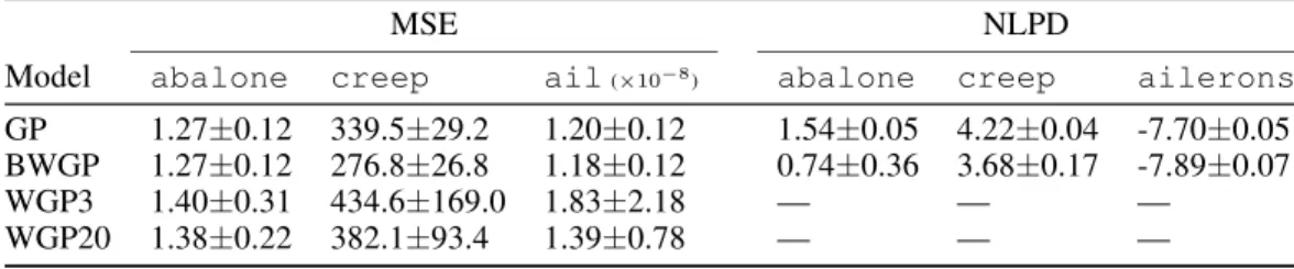
4.3 Censored regression data sets

We will now modify the previous data sets so that they become more challenging. We will consider that they have beencensored, i.e., values that lie above or below some thresholds have been trun-cated. This is a realistic setting in the case of physical measurements (e.g., due to the limitation of measuring devices), but clusters of values lying at the end of the range can appear in other cases. In our experiments, we truncated the upper and lower 20% of the previous datasets, while keeping the remaining 60% of data untouched. Note that the methods have no information about the existing truncation or the used thresholds.

As discussed in [1], for this type of data, WGP tries to spread the samples in latent space by using a very sharp warping function and this causes the model problems. Additionally, the computation of the NLPD becomes erroneous due to numerical problems, with some of thetanhfunctions becom-ing very close tosignfunctions. None of these problems were experienced by BWGP, which still works significantly better than a standard GP on this type of problems, see Table 2. The correspond-ing warpcorrespond-ing functions are displayed on Figs. 3.(e)-(g).

Table 2: NMSE and NLPD figures for the compared methods on censored data sets.

MSE NLPD

Model abalone creep ail(×10−8

) abalone creep ailerons

GP 1.27±0.12 339.5±29.2 1.20±0.12 1.54±0.05 4.22±0.04 -7.70±0.05 BWGP 1.27±0.12 276.8±26.8 1.18±0.12 0.74±0.36 3.68±0.17 -7.89±0.07

WGP3 1.40±0.31 434.6±169.0 1.83±2.18 — — —

WGP20 1.38±0.22 382.1±93.4 1.39±0.78 — — —

4.4 Classification data sets

Classification can be regarded as an extreme case of censoring or quantisation of a regression data set. We also mentioned in Section 2.2 that the (conditional) generative model of GP classification

−15 −10 −5 0 5 10 −10 −5 0 5 10 15 20 25 f g(f) Abalone

(a)abalone(reg)

−200 −100 0 100 200 300 0 100 200 300 400 500 600 f g(f) Creep

(b)creep(reg)

−20 −15 −10 −5 0 5 x 10−4

−3 −2.5 −2 −1.5 −1 −0.5 0x 10−3

f

g(f)

Ailerons

(c)ailerons(reg)

−1 −0.5 0 0.5 1 −1.5 −1 −0.5 0 0.5 1 1.5 f g(f) german

(d)german(class)

−4 −3 −2 −1 0 1 2 3 4 5 −2 −1.5 −1 −0.5 0 0.5 1 1.5 2 2.5 f g(f) Abalone

(e)abalone(cens)

−100 −50 0 50 100 60 80 100 120 140 160 180 200 220 240 f g(f) Creep

(f)creep(cens)

−3 −2 −1 0 1 2 3 4 5 x 10−4

−12 −11 −10 −9 −8 −7 −6 −5 −4x 10

−4

f

g(f)

Ailerons

(g)ailerons(cens)

−0.8 −0.6 −0.4 −0.2 0 0.2 0.4 0.6 0.8 −1.5 −1 −0.5 0 0.5 1 1.5 f g(f) titanic

(h)titanic(class)

Figure 3: Inferred warping functions.

Table 3: Error rates (in percentage) for the proposed model on the benchmark from R¨atsch [18].

ban bre dia fla ger hea ima rin spl thy tit two wav

GP 13.2 29.6 28.0 39.1 27.6 28.6 03.2 21.1 23.4 13.7 23.6 10.1 15.5 BWGP 10.7 29.5 24.5 33.3 23.9 23.5 02.1 04.8 17.0 04.7 22.0 04.2 12.4 GPC 10.6 29.5 24.2 33.5 24.8 21.7 02.1 07.9 22.8 04.0 22.2 04.2 11.4

could be seen as a particular selection forg(f). So we decided to test the BWGP model on the 13 classification data sets from R¨atsch benchmark [18].

Since WGP does not produce any meaningful results on this type of data, as mentioned in [1], we did not include it in the comparison. Instead, we used a standard GP classifier (GPC) using a probit likelihood and expectation propagation for approximate inference. We measured the error rate, which is the performance figure we are interested in for those data sets, averaging over 10 splits of the data. Results from Table 3 show that BWGP is able to match and occasionally exceed the performance of GPC, outperforming in all cases the standard GP. The learned warping functions look similar for the different data sets. We have depicted two typical cases in Figs. 3.(d) and 3.(h). Specially good results are obtained forgerman,ringnorm, andsplice, though we are aware than even better results can be obtained by using an isotropic SE covariance on these data sets [19].

5

Discussion and further work

In this work we have shown how it is possible to variationally integrate out the warping function from warped GPs. This is useful to overcome the limitations of maximum likelihood warped GPs, namely: To work in the low data sample regime; to handle censored observations and classification data; to explicitly model output noise; and to allow for warping functions of unlimited flexibility, which may include flat regions. The experiments demonstrate the improved robustness of the BWGP model, which is able to operate properly in a much wider set of scenarios. While a specific model (should it exist) will generally be a better tool for a specific task (e.g., GPC for classification), BWGP behaves as a Swiss Army knife providing good performance on general tasks.

In addition to the tasks discussed in this work, there are other cases in which BWGP can be of immediate application. One example is ordinal regression [8], where the locations and widths of the bins can be integrated out instead of selected. Another potential future application is within the popular field of copulas [20, 21, 22, 23], since they routinely resort to fixed warpings of GPs. Acknowledgments

References

[1] E. Snelson, Z. Ghahramani, and C. Rasmussen. Warped Gaussian processes. InAdvances in Neural Information Processing Systems 16, 2003.

[2] C. E. Rasmussen.Evaluation of Gaussian Processes and other Methods for Non-linear Regression. PhD thesis, University of Toronto, 1996.

[3] M.N. Gibbs.Bayesian Gaussian Processes for Regression and Classification. PhD thesis, University of Cambridge, 1997.

[4] C.E. Rasmussen and C.K.I. Williams.Gaussian Processes for Machine Learning. Adaptive Computation and Machine Learning. MIT Press, 2006.

[5] M.N. Schmidt. Function factorization using warped gaussian processes. InProc. of the 26th International Conference on Machine Learning, pages 21–928. Omnipress, 2009.

[6] Y. Zhang and D.-Y Yeung. Multi-task warped gaussian process for personalized age estimation. InIEEE Conf. on Computer Vision and Pattern Recognition, pages 2622–2629.

[7] C.K.I. Williams and C.E. Rasmussen. Gaussian processes for regression. InAdvances in Neural Infor-mation Processing Systems 8. MIT Press, 1996.

[8] W. Chu and Z. Ghahramani. Gaussian processes for ordinal regression. Journal of Machine Learning Research, 6:1019–1041, 2005.

[9] M.K. Titsias and N.D. Lawrence. Bayesian Gaussian process latent variable model. InProc. of the 13th International Workshop on Artificial Intelligence and Statistics, volume 9 ofJMLR: W&CP, pages 844–851, 2010.

[10] M.K. Titsias. Variational learning of inducing variables in sparse Gaussian processes. InProc. of the 12th International Workshop on Artificial Intelligence and Statistics, 2009.

[11] M. L´azaro-Gredilla and M. Titsias. Variational heteroscedastic Gaussian process regression. In28th International Conference on Machine Learning (ICML-11), pages 841–848, New York, NY, USA, June 2011. ACM.

[12] M. Opper and C. Archambeau. The variational Gaussian approximation revisited. Neural Computation, 21(3):786–792, 2009.

[13] M.K. Titsias A.C. Damianou and N.D. Lawrence. Variational gaussian process dynamical systems. In

Advances in Neural Information Processing System 25. IEEE Conf. publications, 2011.

[14] A. Frank and A. Asuncion. UCI machine learning repository, 2010. http://archive.ics.uci.

edu/mlUniversity of California, Irvine, School of Information and Computer Sciences.

[15] Materials algorithms project (MAP) program and data library. http://www.msm.cam.ac.uk/

map/map.html.

[16] D. Cole, C. Martin-Moran, A. G. Sheard, H. K. D. H. Bhadeshia, and D. J. C. MacKay. Modelling creep rupture strength of ferritic steel welds.Science and Technology of Welding and Joining, 5:81–90, 2000. [17] L. Torgo.http://www.liacc.up.pt/˜ltorgo/Regression/.

[18] G. R¨atsch, T. Onoda, and K.-R. M¨uller. Soft margins for AdaBoost. Machine Learning, 42(3):287– 320, 2001. http://people.tuebingen.mpg.de/vipin/www.fml.tuebingen.mpg.de/

Members/raetsch/benchmark.1.html.

[19] A. Naish-Guzman and S. Holden. The generalized FITC approximation. InAdvances in Neural Informa-tion Processing Systems 20, pages 1057–1064. MIT Press, 2008.

[20] R.B. Nelsen.An Introduction to Copulas. Springer, 1999.

[21] P.X.-K. Song. Multivariate dispersion models generated from Gaussian copula.Scandinavian Journal of Statistics, 27(2):305–320, 2000.

[22] A. Wilson and Z. Ghahramani. Copula processes. InAdvances in Neural Information Processing Systems 23, pages 2460–2468. MIT Press, 2010.

[23] F.L. Wauthier and M.I. Jordan. Heavy-tailed process priors for selective shrinkage. InAdvances in Neural Information Processing Systems 23. MIT Press, 2010.