Smoothing Parameter Selection for Nonparametric Regression Using Smoothing Spline

Vol. 6, No. 2, 2013, 222-238

ISSN 1307-5543 – www.ejpam.com

Smoothing Parameter Selection for Nonparametric Regression

Using Smoothing Spline

Dursun Aydin

_{, Memmedaga Memmedli}

_{, Rabia Ece Omay}

1_{Department of Statistics, Mugla Sitki Kocman University 48000 Mugla, Turkey} 2_{Department of Statistics, Anadolu University 26470 Eskisehir, Turkey}

Abstract. In this paper, the smoothing parameter selection problem has been examined in respect to a smoothing spline implementation in predicting nonparametric regression models. For this purpose, a simulation study has been performed by using a program written in MATLAB. The simulation study provides a comparison of the nine smoothing parameter selection methods. In this connection, 500 replications have been performed in simulation for sample sets with different sizes. Thus, the appro-priate selection criteria are provided for a suitable smoothing parameter selection.

2010 Mathematics Subject Classifications: 62E17, 65C05, 65C20, 65C60

Key Words and Phrases: Nonparametric regression, Smoothing spline, Smoothing parameter,

Selec-tion criteria, Generalized cross validaSelec-tion.

1. Introduction

Smoothing spline method is one of the most popular methods used for the prediction of the nonparametric regression models. The role of this method is to estimate the nonparametric function that minimizes penalized least squares criterion. A roughness penalty term multiplied by a positive smoothing parameter is added to the residual sum of squares in smoothing spline regression. In the light of this approach, the estimation of the unknown function depends on smoothing parameterλ. Therefore, the determination of an optimum smoothing parameter in the interval(0,∞)was found to be an underlying complication. In the literature, different selection methods are components of various studies for an appropriate smoothing parameter. Indeed, to a considerable extent, Craven and Wahba[5], Hardle[8], Hardle, Hall and Marron [9], Wahba[26], Hurvich, et al. [11], Eubank[6], Lee and Solo[17], Hastie and Tibshirani [10], Schimek[22], Cantoni and Ronchetti[4], Ruppert, Wand and Carroll[21], Lee[15, 16], and Kou[12]supplement on the selection of the smoothing parameter.

In this study, the empirical performances of the selection methods used in selection of the smoothing parameter are compared. Selection methods used in our simulation study are an

∗_{Corresponding author.}

Email addresses:[email protected](D. Aydin)

improved version of Akaike information criterion (AICc), robustified cross-validation (RCV), average predictive square error (PSE), parallel of Akaike’s information criterion (GFAIC), gen-eralized cross-validation (GCV), cross-validation (CV), Mallows’ Cp criterion,risk estimation using classical pilots (RCP) and local risk estimation (LRS). A simulation study was conducted to find out which selection methods are the best in smoothing parameter selection. To throw light on this issue, the samples differing in small and large sizes are secured by means of the above mentioned simulation, and moreover, nine selection methods are evaluated.

This paper is mainly concerned with the selection of smoothing parameter (or penalty pa-rameter) through Monte Carlo simulation study. Smoothing parameters play a crucial role in this procedure. These parameters are said to control the trade off between fidelity to the data and smoothness: too low values of smoothing parameter overfit the data, whereas too high values oversmooth. Krivobokova and Kauermann[14]showed that using the REML to esti-mate smoothing parameter outperforms other methods such as (generalized) CV or Akaike criterion especially when the error correlation structure is misspecified. Krivobokova et al. [13]formulated a hierarchical mixed model to estimate local smoothing parameter to achieve adaptive penalized spline smoothing. Yanrong Cao et al. [27]discussed different methods of choosing the important smoothing parameter and recommend GCV as the choice for penal-ized spline smoothing parameter selection for both computational efficiency and accuracy of the functional coefficient regression models. Aydin and Memmedli [3] recommended GCV and REML as being good smoothing parameter selection criteria for small and medium sized samples.

Nonparametric regression and its prediction are discussed in section 2. Section 3 reviews nine different smoothing parameter selection methods. Section 4 compares these methods via a simulation study, and finally, the conclusion and recommendations are presented in section 5.

2. Nonparametric Regression Model and its Prediction

Nonparametric regression model including a predictor (independent) variable and a re-sponse variable is defined as

yi= f(xi) +"i, a<x1<...<xn< b (1)

where f ∈ C2[a,b] is an unknown smooth function, (y_i)n_i=1 are observation values of the response variable y,(xi)ni=1are observation values of the predictor variable x and("i)ni=1are normal distributed random errors with zero mean and common varianceσ2 ("_i˜N(0,σ2)).

The basic aim of the nonparametric regression is to estimate unknown function f ∈ C2[a,b](the class of all functions f with continuous first and second derivatives) in model (1). Smoothing spline estimate of the f function appears as a solution to the following mini-mization problem: Find fˆ∈C2[a,b]that minimizes the penalized residual sum of squares

S(f) = n

X

i=1

y_i−f(x_i) 2+λ b

Z

a

for pre-specified valueλ >0. The first term in equation (2) denotes the residual sum of the squares (RSS) and it penalizes the lack of fit. The second term which is weighted byλdenotes the roughness penalty and it imposes a penalty on roughness. In other words, it penalizes the curvature of the function f. Theλin (2) is recognized to be the smoothing parameter. Asλ varies from 0 to+, the solution varies from interpolation to a linear model. Asλ→+∞, the roughness penalty dominates in (2) and the spline estimate is compelled to be a constant. As λ→→0, the roughness penalty disappears in (2) and the spline estimation interpolates the data. Thus, the smoothing parameterλplays a key role in controlling the trade-off between

the goodness of fit represented by n

P

i=1

y_i−f(x_i) 2and smoothness of the estimate measured

by b

R

a

f00(x) 2d x.

The solution based on smoothing spline for minimum problem in the equation (2) is known as a “natural cubic spline” with knots at x₁, . . . ,x_n. From this point of view, a special structured spline interpolation which depends on a chosen valueλ develops into a suitable approach of function f in model 1. Let f = (f(x1), . . . ,f(xn)) be the vector of values of function f at the knot points x₁, . . . ,x_n. The smoothing spline estimate ˆfλ of this vector or

the fitted values for data y = (y₁, . . . ,y_n)T are projected by

ˆ_f λ=       ˆ

f_λ(x₁) ˆ

f_λ(x₂) .. . ˆ

fλ(xn)

     

(n×1) =Sλ

      y1 y₂ .. . y_n      

(n×1)

orˆfλ=Sλy (3)

where fˆλ is a natural cubic spline with knots at x1, . . . ,xn for a fixed λ > 0, and Sλ is

a well-known positive-definite (symmetrical) smoother matrix which depends on λ and the knot points x1, . . . ,xn, but not on y. Function fˆλ, the estimation of function f, is obtained by

cubic spline interpolation that rests on condition fˆ(x_i) = ( ˆf)_i, i=1, 2, . . . ,n. To gain better perspective on smoothing spline, Eubank[6], Green and Silverman[7]and Wahba[26]state studied opinions.

3. Smoothing Parameter Selection Methods

3.1. Selection Methods used in Simulation Study

Various smoothing parameter selection methods are featured in the literature. Most of these suggested methods were implemented in our simulation study. Moreover, a selection criterion from previous studies in the literature to provide an effective performance was also introduced in this particular study. The selection criteria used in our simulation study are classified as:

Average predictive squared error: In selection the smoothing parameter, it is essential not to try to minimize the mean squared error at each x_i, but instead, the focus should centre on a global measures such as average predictive squared error

PS E(λ) =

¨

1+ t r(SλS T λ)

n «

σ2+

(I−S_λ)f

2

n (4)

Wheret r(SλS_λT)is trace of matrixSλS_λT and

(I−S_λ)f

is norm of matrix(I−S_λ)f. Ifσ2is

not known, in practice an estimation forσ2can be given by

ˆ

σ2= RSS(λ ∗₎

n−t r 2Sλ∗−Sλ∗STλ∗ =

(S_λ∗−I)y

2

n−t r 2Sλ∗−Sλ∗STλ∗

,

whereRSS(λ∗)is the residual sum of square from a smoothS_λ∗y andλ∗is a pilotλselected by any selection methods[see 10].

Cross-Validation:The basic idea of CV is to disregard one of the points

x_i,y_i n_i=1 sequen-tially, to select the smoothing parameterλ that minimizes the residual sum of squares, and to estimate the squared residual for a smooth function at xi based on the remaining(n−1) points. The CV score can be translated as

CV(λ) = 1

n

n

X

i=1

n yi−fˆ

(−i) λ (xi)

o2

≡CV(λ) = 1

n

n

X

i=1

¨

y_i−fˆ_λ(x_i) 1−(S_λ)_ii

«2

, (5)

where fˆλ is the fit (spline smoother) for n pairs of measurements

xi,yi

n

i=1with smoothing parameterλ, and fˆ_λ(−i)is the fit calculated by leaving out the ith data point and(Sλ)ii is the ith diagonal element of smoother matrixSλ [see 26, 7].

Using the approximations (S_λ)_ii ≈ ¦S_λS_λT©

ii and 1/ 1−(Sλ)ii

2

≈1+2(S_λ)_ii, signifies

thatE{C V(λ)} ≈PS E(λ) +2/n+ n

P

i=1

(Sλ)iib2i(λ)[see 10].

be procured as follow[see 5, 26]:

GC V(λ) = 1

n

n

P

i=1

¦

y_i−fˆλ(x1)

©2

1−n−1t r(Sλ) 2 =

n−1 I−S_λy

2

n−1t r I−Sλ

2 (6)

Mallows’ CP criterion: In the literature, C_p criterion is referred to as an unbiased risk estimate (UBR). This type of estimate was suggested by Mallows[18]in the regression case, and applied to smoothing spline by Craven and Wahba[5]. Ifσ2 is recognized, an unbiased estimate of the residual sum of squares is provided byC_p criterion:

Cp(λ) = 1

n n

(S_λ−I)y

2

+2σ2t r(Sλ)−σ2

o

= 1

n n

y−fˆ_λ

2

+2σ2t r(Sλ)−σ2

o

(7)

Unlessσ2is known, in practice an estimation forσ2 can be given by

ˆ

σ2= ˆσ2_ˆλ= n

P

i=1

€

y_i−fˆ_λˆ(xi)

Š2

t r I−S_λˆ =

(S_λˆ−I)y

2

t r I−S_λˆ

(8)

where λˆ is pre-chosen with any of the CV, GCV or AICC criteria (λˆ is an estimate of λ) For reference, see[15, 16, 26]. According to Hastie and Tibshirani[10]and Ruppert, et. al.[21], GCV is approximately equal toC_p.

Improved Akaike information criterion:An improved version of a criterion based on the classical Akaike information criterion (AIC), AICc criterion, is used for choosing the smoothing parameter for nonparametric smoothers[11]. This improved criterion is defined as

AI C_C(λ) =log

P ¦

y_i−fˆ_λ(x_i)©2

n +1+

2

t r(S_λ) +1

n−t r(S_λ)−2

=log

S_λ−Iy

2

n +1+

2t r(Sλ) +1

n−t r(Sλ)−2

. (9)

This criterion is easy to apply for the selection of smoothing parameter, as can be seen from the equation (9).

Robustified Cross-Validation: The smoothing parameterλcan be chosen by method of robustified cross-validation (RCV). This serves to reduce risk of smoothing parameter mis-specification in small sample sizes. Most of the selections methods have been proposed to optimizeλare related to a distributional. RCV criterion that does not refer to a distributional assumption is proposed by Robinson and Moyeed[20]. Robustified cross-validation score is given by

RC V(λ) =n−1 1+n

−1_{+t r S} λ2

1+n−1+t r Sλ

2

I−S_λy

2

. (10)

Parallel of Akaike’s information criterion: A result of Stone [24] states that in the case of independent observation, the sum over i of the values of log-likelihood function in

y = (y₁, . . . ,y_n)with parameters estimated by maximum likelihood based on

x_i is asymp-totically equivalent to Akaike’s information criterion (AIC). This result is not directly applica-ble to splines, instead of a simple, maximum-likelihood estimate and σ2 as additional noise parameter has to be taken into account. However, there is parallel of AIC[22]. This parallel criterion is given by

G F_{AI C} =n−1 I−S_λy

2

+exp(2n−1t r(S_λ)) (11)

Minimization ofG FAI C looks like maximization of the log-likelihood function in y.

Risk estimation using classical pilots: Risk function measures the distance between the actual regression function (f) and its estimation (fˆ_λ). Needless to say that, a good estimate must contain minimum risk. A direct computation leads to the bias-variance decomposition forR(f,fˆλ):

R(f,fˆ_λ) = 1

nE

f −fˆ_λ

2 = 1 n n

S_λ−If

2

+σ2t r(S_λS_λT)o (12)

A clear-cut explanation shows that R(f,fˆ_λ) = E¦C_p(λ)©. Because the risk R(f,fˆ_λ) is an unknown quantity, so-called risk is now estimated by computable quantity R( ˆfλp,fˆλ). The

obtained expression forR( ˆf_λ p,

ˆ

f_λ)is

R( ˆfλp,

ˆ

fλ) =

1

nE fˆλp−

ˆ fλ 2 = 1 n Sλ−I

_ˆ

fλp

2 + ˆσ2_λ

pt r(SλS

T λ)

, (13)

whereσˆ2_λ

p and

ˆ

f_λ

p are the appropriate pilot estimates forσ

2 _{andf, respectively. The pilotλ} p selected by classical methods is used for computation of the pilot estimates.

Local risk estimation: The LRS method proposed by Lee[16], aims to select the ˆf_λ(x_i) that minimizes the local riskR_λ(x_i) =E¦f(x_i)− ˆf_λ(x_i)©2for the each knot pointsx_i A direct computation leads to the bias-variance decomposition forRλ(xi):

Rλ(xi) =

Sλf(xi)−f(xi) 2

+σ2sλ(xi) (14)

In the above equation, S_λf

(x_i)is the ith element of vectorS_λf ands_λ(x_i)is the ith diagonal element of the square matrixSλSλT. An estimator forRλ(xi)is firstly computed and the ˆfλ(xi) is selected in order to minimizes it. This process is repeated for all x_i’s and at the end of the process a final mixed estimate for f is derived. The LRS method can be practically performed with the following five steps[15]:

(i) For a set of pre-selected smoothing parametersλ₁<. . .< λ_m, calculate the correspond-ing set of smoothcorrespond-ing spline estimates: F=¦fˆλ1, . . . ,

ˆ

fλm ©

;

(ii) Select the pilot valueλ_pfromAI C_c criterion in (9) by using the elements inF;

(iii) Forλ_p, calculate the estimates fˆλp, andσˆ

2

(iv) Substitute the pilots ˆfλp andσˆ

2

λp into the expression

ˆ

Rλ(xi) =

n Sλfˆλp

(x_i)₋ ˆfλp(xi) o2

+ ˆσ2_λ

psλ(xi)

and obtain the estimatesˆR_λ(x_i)

(v) For eachx_i, find thefˆλ(xi)fromF which minimizesRˆλ(xi)and the final estimate accept the appropriate values ˆf_λ(x_i)for f(x_i)

3.2. Other Selection Methods

We also explored most of the selection methods that are not used in our simulation. Har-dle, Hall and Marron[9]recommended thatAI C(λ), F P E(λ), andSH(λ)should not be used because of their trivial minimum at the no-smoothing point. They are also preference T(λ) for bandwidth selector, but the statement of Rice[19]that “these result are suggestive”, but

T(λ)hasn’t had a good performance in our simulation study. It is accepted thatG L M(λ) es-timates undersmooths relative to the GC V(λ) estimate (see, Wahba[25]). Moreover, Hastie and Tibshirani [10], also point out that minimizing ASR(λ) over the smoothing parameter leads to an interpolation estimate.

Furthermore, we have also performed a simulation study for all the selection methods. In such cases, the selection methods produced invalidating results when compared with the selection methods such as AICc, GFAIC, GCV, Cp and RCV used in our simulation study. For this reason, in this paper, the simulation results of theAI C,F P E,SH,T,G L MandASRcriteria are not displayed. For smoothing spline, these selection criteria can be given as:

(a) Akaike’s information criterion[2],

AI C(λ) = 1

n

I−S_λy

2

exp(1₋n−1t r(Sλ));

(b) finite prediction error[1],

F P E(λ) = 1

n

I−S_λy

21+n−1t r(Sλ)

1−n−1_{t r(S} λ)

;

(c) a model selector of[23];

SH(λ) = 1

n

I−S_λy

2€

1−n−12t r(Sλ)

Š

(d) Rice’s T criterion[19];

T(λ) = 1

n

I−S_λy

2

/€1₋n−12t r(Sλ)

(e) A generalization of the maximum likelihood (GLM),

G L M(λ) = y0 I−S_λ

y/”det+ I−S_λ—1/n−m

;

where det+ I−Sλis the product of n−mnonzero eigenvalues of I−Sλ.

(f) Average squared residual,

ASR(λ) = 1

n

n

X

i=1

¦

yi−fˆλ(xi)

©

2

.

4. Simulation Study

This section reports the results of a Monte Carlo simulation study. This study was con-ducted to evaluate the performances of the nine selection methods mentioned above. The experimental setup in this paper is adopted from Professor Steve Marron. By using a program coded in MATLAB, we generated the samples sized n=25, 50, 100, 150, 200, 350, 400. The number of replications was 500 for each of the samples. For each simulated data sets, the mean squared-errors (MSE) was used for evaluate the quality of any curve estimate fˆ. To find out if the difference between the MSE median values of any two selection methods is signifi-cant or not, the paired Wilcoxon tests were assessed. In this way, methods which complement the best smoothing parameter were determined by evaluating so-called selection methods.

4.1. Experimental Plan and Generation of the Data

The experimental setup applied at this stage was designed to study the effects of the following three factors which vary an independent and effective approach: Noise level; Spatial variation; Variance function.

The setup specification is listed Table 1. The simulation study was performed according to MATLAB program, and the experimental setup was designed in the following framework:

• Totally three sets of numerical experiments were performed. For each set of experi-ments, only one of the above three experimental factors (e.g., noise level, degree of spatial variation and noise variance function) has been altered while the remaining two have been kept unchanged.

• Within each set of experiments, the factor levels was modified four times (i.e., r = 1, 2, 3, 4) to detect the effects of any experimental factor in Table 1.

• To see the performance of the small and large samples of the selection methods. For each factor level r within each set of experiments, we generated 7 different samples with sample sizesn=25, 50, 100, 150, 200, 350, 400.

• We computed the appropriate smoothing spline estimatorsfˆλin equality (3) by selecting

the smoothing parameterλwhich minimizes the selection methods.

• We used the MSE values to evaluate fˆλ computed according to each of the selection

criterion: M S E = 1 n

n

P

i=1

¦

f(x_i)₋ ˆfλ(xi)

©2

, (fˆλ(xi) = ( ˆfλ)i), (where f(xi) is value at

knots x_i of the appropriate function f defined in Table 1)

• Paired Wilcoxon test was applied to test whether MSE values was considered as the performance measure of any two methods are significant or not.

• The factor levels indicated as r was changed four times (i.e., r =1, 2, 3, 4) in order to detect the effects of any factor from three factors in Table 1.

• By considering 3 factors, 4 factor levels and 7 samples, totally, 84 numerical experiments were conducted.

Table 1: Averaged Wilcoxon test ranking values for the nine selection methods in small sample sizes

Factors Generic Form Particular Choices

Noise Level y_{i r}= f(x_i) +σ_r"_i Factors

Spatial variation y_{i r}= f(x_i) +σ_r"_i σ=0.2, f_r(x) =px(1−x)sin2π{1+2(9−4r)/5} x+2(9−4r)/5

Variance function y_{i r} = f(x_i) +pv_r(x_i)"_i v_r(x) = [0.15{1+0.4(2r−7)(x−0.5)}]2

r=1, . . . , 4;x_i= i−_n0.5;"_i∼iid N(0, 1);f(x) =1.5θ€x−_0.150.35Š−θx_0.04−0.8;θ(u) = p1 2πexp

−u2 2

n=25, 50, 100, 200, 350, 400 (it was taken seven sample size).

4.2. Experimental Evaluations

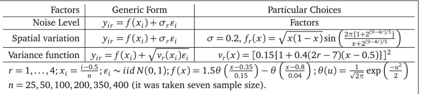
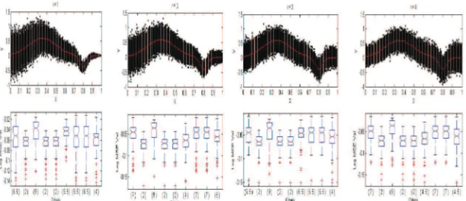
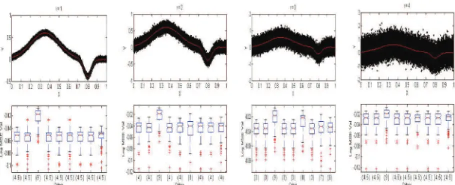
For each simulated data set used in the experiments, the MSE values were used in order to evaluate the quality of any curve estimate fˆ. Paired Wilcoxon tests were applied to test whether the difference between the median MSE values of any two methods is significant or not. The significance level used was 5%. The selection methods were also ranked as follows: If median MSE value of a method is significantly less than the remaining five, it will be assigned a rank 1. If median MSE value of a method is significantly larger than one but less than the remaining four, it will be assigned a rank 2, and similarly for ranks 3-9. Methods having non-significantly different median values will share the same averaged rank, on the other hand, method or methods having the smallest rank will be superior.

right, AICc, RCV, FSE, GFAIC, GCV, CV, Cp, RCP and LRS. The numbers below the boxplots are the paired Wilcoxon test rankings. For 84 different simulation experiments, the averaged ranking values of the selection methods according to Wilcoxon tests are tabulated in Tables A1 and A2. All results tables are shown in the appendix;(∗)indicates the selection methods with the best rankings.

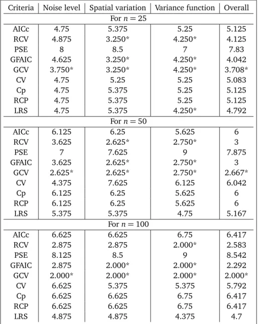
According to the results in Table A1, for small sized samples (for n=25, 50, 100), GCV has had the best empirical performance for all factors. Furthermore, GFAIC and RCV have shared the better performance after GCV criterion. In accordance with the overall Wilcoxon test rankings in Table A1, GCV, GFAIC and RCV have also displayed a good performance. As shown Table A1, because ofR€f,fˆλ

Š

=E¦C_p(λ)©, C_pand RCP methods produced the same results under all experimental factors. In this situation, for small sample sizes, for which reason the effects of the replication of simulation, Cp is approximately equal to its E

¦ Cp

©

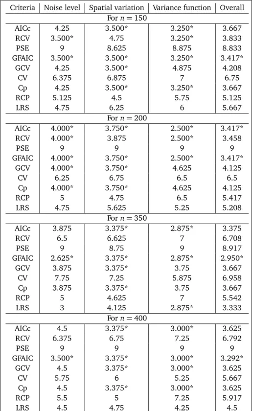
. For small samples, it is observed that PSE has produced the worst performance. According to Table A2, for large sized samples (forn=150, 200, 350400), GFAIC criterion has had the best empirical performance. Generally it is shown that AICc, RCV and GCV (Cp) criteria have shared a better performance after than GFAIC. According to the overall Wilcoxon test rankings in Table A2, GFAIC, AICc and RCV criteria can be ranked in terms of the performance. As shown in Table A2, generally, Cp and GCV gave the same results. This can be interpreted to follow the accepted view that GCV is asymptotically equal to GCV[see 10]. That is to say that, for large sized samples, because of the effect of the replication of simulation, performance of the GCV and Cp is approximately equal. PSE has also produced the worst performance for large samples.

5. Conclusion and recommendations

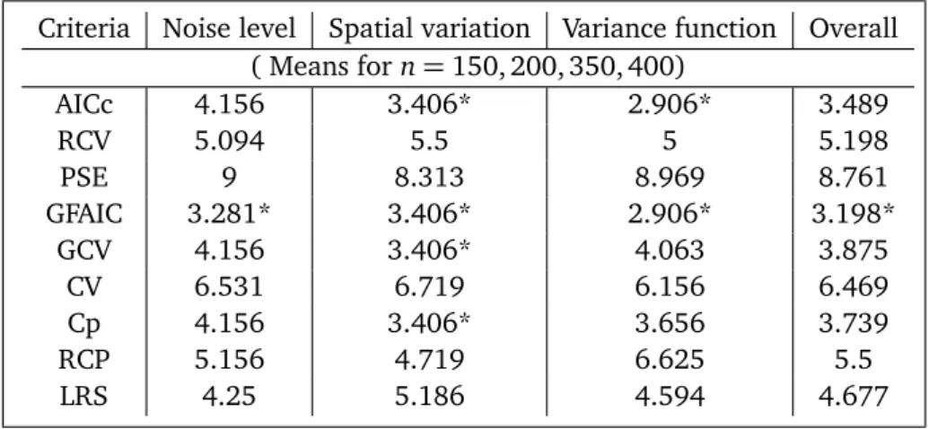
The scores in Tables A3 and A4 in the appendix are obtained by taking the means of the averaged Wilcoxon test ranking values tie with each of the selection methods in Table A1-A2 respectively.

As shown in Table A3, according to the means of the small samples for all factors, GCV,

G F_{AI C} and RCV criteria have had the best empirical performance respectively. When it is compared to the other criteria, PSE,Cp(RCP),AI Cccriteria have resulted in the worst perfor-mance.

According to the means of the large samples for all factors in Table A4, it is observed that GFAIC,AI Cc, GCV (Cp) have had the best empirical performance. However, PSE and CV have produced the worst result

Finally, by considering the simulation results and evaluations given in the above, the fol-lowing suggestions have to be taken into account:

• For both large and small samples, G F_{AI C} and GCV are recommended as being the best selection criteria;

• For large samples, the implementation ofAI C_ccriterion, in addition to GFAIC and GCV (C_p) criteria would be more beneficial. For small samples, RCV criterion in addition to GFAIC and GCV criteria should prove fruitful.

Naturally, the above recommended suggestions have to be considered with a fair amount of caution as they are only an appraisal based on simulation results.

References

[1] H Akaike. Statistical predictor identification. Annals of the Institute of Statistical

Mathe-matics (AISM), 22:203–217, 1970.

[2] H Akaike. A new look at the statistical model identification. IEEE Transactions on

Auto-matic Control, 19(6):716–723, 1974.

[3] D Aydin and M Memmedli. Optimum smoothing parameter selection for penalized least squares in form of linear mixed effect models. Optimization, iFirst:1–18, 2011.

[4] E Cantoni and E Ronchetti. Resistant selection of smoothing parameter for smoothing splines. Statisics and Computing, 11:141–146, 2001.

[5] P Craven and G Wahba. Smoothing noisy data with spline functions. Numerische

Math-ematik, 31:377–403, 1979.

[6] R L Eubank. Nonparametric Regression and Smoothing Spline. Marcel Dekker Inc., New York, 1999.

[7] P J Green and B W Silverman. Nonparametric Regression and Generalized Linear Model. Chapman & Hall, New York, USA, 1994.

[8] W Hardle. Applied Nonparametric Regression. Cambridge University Press, Cambridge, 1991.

[9] W Hardle, P Hall, and J S Marron. How far are automatically chosen regression smooth-ing parameters from their optimum? (with discussion). Journal of the American

Statis-tical Association, 83:86–89, 1988.

[10] T Hastie and R J Tibshirani. Generalized Additive Models. Chapman & Hall, London, 1999.

[11] C M Hurvich, J S Simonoff, and C L Tasi. Smoothing parameter selection in nonpara-metric regression using an improved akaike information criterion. Journal of the Royal

Statistical Society. Series B (Statistical Methodology), 60:271–293, 1998.

[12] S C Kou. On the efficiency of selection criteria in spline regression. Probability Theory

[13] T Krivobokova, C M Crainiceanu, and G Kauermann. Fast adaptive penalized splines.

Journal of Computational and Graphical Statistics, 17:1–20, 2008.

[14] T Krivobokova and G Kauermann. A note on penalized spline smoothing with correlated errors.Journal of the American Statistical Association, 102:1328–337, 2007.

[15] T C M Lee. Smoothing parameter selection for smoothing splines: A simulation study.

Computational Statistics & Data Analysis, 42:139–148, 2003.

[16] T C M Lee. Improved smoothing spline regression by combining estimates of different smoothness. Statistics & Probability Letters, 67:133–140, 2004.

[17] T C M Lee and V Solo. Bandwidth selection for local linear regression: A simulation study. Computational Statistics & Data Analysis, 14:515–532, 1999.

[18] C Mallows’. Some comments on cp. Technometrics, 15:661–375, 1973.

[19] J Rice. Bandwidth choice for nonparametric regression. Annals of Statistics, 12:1215– 1230, 1984.

[20] T Robinson and R Moyeed. Making robust the cross-validation choice of smoothing pa-rameter in spline regression.Communications in Statistics - Theory and Methods, 18:523– 539, 1989.

[21] D Ruppert, M P Wand, and R J Carroll.Semiparametric Regression. Cambridge University Press, Cambridge, 2003.

[22] G M Schimek. Smoothing and Regression: Approaches, Computation, and Application. John Willey & Sons, Inc., USA, 2000.

[23] R Shibata. An optimal selection of regression variables.Biometrika, 68(1):45–45, 1981.

[24] M Stone. An asymptotic equivalence of choice of model by cross-validation and akaike’s criterion. Journal of the Royal Statistical Society. Series B (Statistical Methodology), 39:44–47, 1977.

[25] G Wahba. A comparison of gcv and gml for choosing the smoothing parameter in the generalized spline smoothing problem. Annals of Statistics, 13:1378–1402, 1985.

[26] G Wahba. Spline Model For Observational Data. Siam, Philadelphia, 1990.

[27] C Yanrong, Z W Tracy L Haiqun, and Y Yan. Penalized spline estimation for functional coefficient regression models. Computational Statistics and Data Analysis, 54:891–905, 2010.

Figure A1: Simulation results correspond to the noise level factor forn=25.

Figure A2: Simulation results correspond to the spatial variation factor forn=50.

Figure A4: Simulation results correspond to the noise level factor for n=200.

Figure A5: Simulation results correspond to the spatial variation factor forn=350.

Table A1: Averaged Wilcoxon test ranking values for the nine selection methods in small sample sizes

Criteria Noise level Spatial variation Variance function Overall Forn=25

AICc 4.75 5.375 5.25 5.125

RCV 4.875 3.250* 4.250* 4.125

PSE 8 8.5 7 7.83

GFAIC 4.625 3.250* 4.250* 4.042

GCV 3.750* 3.250* 4.250* 3.708*

CV 4.75 5.25 5.25 5.083

Cp 4.75 5.375 5.25 5.125

RCP 4.75 5.375 5.25 5.125

LRS 4.75 5.375 4.250* 4.792

Forn=50

AICc 6.125 6.25 5.625 6

RCV 3.625 2.625* 2.750* 3

PSE 7 7.625 9 7.875

GFAIC 3.625 2.625* 2.750* 3

GCV 2.625* 2.625* 2.750* 2.667*

CV 4.375 7.625 6.125 6.042

Cp 6.125 6.25 5.625 6

RCP 6.125 6.25 5.625 6

LRS 5.375 5.375 4.75 5.167

Forn=100

AICc 6.625 6.625 6.75 6.417

RCV 2.875 2.875 2.000* 2.583

PSE 8.125 8.5 9 8.542

GFAIC 2.875 2.000* 2.000* 2.292

GCV 2.000* 2.000* 2.000* 2.000*

CV 6.625 5.375 5.375 5.792

Cp 6.625 6.625 6.75 6.417

RCP 6.625 6.625 6.75 6.417

Table A2: Averaged Wilcoxon test ranking values for the nine selection methods in large sample sizes

Criteria Noise level Spatial variation Variance function Overall Forn=150

AICc 4.25 3.500* 3.250* 3.667

RCV 3.500* 4.75 3.250* 3.833

PSE 9 8.625 8.875 8.833

GFAIC 3.500* 3.500* 3.250* 3.417*

GCV 4.25 3.500* 4.875 4.208

CV 6.375 6.875 7 6.75

Cp 4.25 3.500* 3.250* 3.667

RCP 5.125 4.5 5.75 5.125

LRS 4.75 6.25 6 5.667

Forn=200

AICc 4.000* 3.750* 2.500* 3.417*

RCV 4.000* 3.875 2.500* 3.458

PSE 9 9 9 9

GFAIC 4.000* 3.750* 2.500* 3.417*

GCV 4.000* 3.750* 4.625 4.125

CV 6.25 6.75 6.5 6.5

Cp 4.000* 3.750* 4.625 4.125

RCP 5 4.75 6.5 5.417

LRS 4.75 5.625 5.25 5.208

Forn=350

AICc 3.875 3.375* 2.875* 3.375

RCV 6.5 6.625 7 6.708

PSE 9 8.75 9 8.917

GFAIC 2.625* 3.375* 2.875* 2.950*

GCV 3.875 3.375* 3.75 3.667

CV 7.75 7.25 5.875 6.958

Cp 3.875 3.375* 3.75 3.667

RCP 5 4.625 7 5.542

LRS 3 4.125 2.875* 3.333

Forn=400

AICc 4.5 3.375* 3.000* 3.625

RCV 6.375 6.75 7.25 6.792

PSE 9 9 9 9

GFAIC 3.500* 3.375* 3.000* 3.292*

GCV 4.5 3.375* 3.000* 3.625

CV 5.75 6 5.25 5.667

Cp 4.5 3.375* 3.000* 3.625

RCP 5.5 5 7.25 5.917

Table A3: Means of the averaged Wilcoxon test ranking values for the nine selection methods

Criteria Noise level Spatial variation Variance function Overall ( Means for n=25, 50, 100)

AICc 5.667 5.958 5.875 5.833

RCV 3.792 2.917 3.000* 3.236

PSE 7.708 8.208 8.333 8.083

GFAIC 3.708 2.625* 3.000* 3.111

GCV 2.792* 2.625* 3.000* 2.806*

CV 5.125 6.083 5.583 5.597

Cp 5.667 6.083 5.875 5.875

RCP 5.667 6.083 5.875 5.875

LRS 5 5.208 4.458 4.889

Table A4: Means of the averaged Wilcoxon test ranking values for the nine selection methods

Criteria Noise level Spatial variation Variance function Overall ( Means forn=150, 200, 350, 400)

AICc 4.156 3.406* 2.906* 3.489

RCV 5.094 5.5 5 5.198

PSE 9 8.313 8.969 8.761

GFAIC 3.281* 3.406* 2.906* 3.198*

GCV 4.156 3.406* 4.063 3.875

CV 6.531 6.719 6.156 6.469

Cp 4.156 3.406* 3.656 3.739

RCP 5.156 4.719 6.625 5.5