Hungarian Association of Agricultural Informatics European Federation for Information Technology in Agriculture, Food and the Environment
Journal of Agricultural Informatics. 2015 Vol. 6, No. 2 journal.magisz.org
Analyzing the value of the residue of crops grown on arable land with stochastic
optimization
Ádám Zlatniczki 1
I N F O
Received 17 March 2015 Accepted 16 Apr 2015 Available on-line 29 Jun 2015 Responsible Editor: M. Herdon
Keywords:
value of crop residue, optimal artificial fertilizer allocation, stochastic optimization, Monte Carlo simulation, linear programming
A B S T R A C T
Determining the value of the residues of crops grown on arable land is a non-trivial task, depending much on how it is defined. In this paper the value of residues is considered to be the savings achieved on the total expense of artificial fertilizer distribution by returning the residues into the soil. A general linear programming approach is presented to obtain optimal artificial fertilizer allocation. Since the amount of artificial fertilizers required depends on uncertain inputs Monte Carlo simulation is applied in conjunction with linear programming to solve the arising stochastic optimization problem. The input data, such as the national average yield, specific amounts of nutrients required by crops to achieve the national average yield and publicly available details of different artificial fertilizer products are specific to Hungary, but the mathematical model presented is general in nature. Simulations are executed for some of the major crops, including wheat, corn, sunflower and rape. The distribution of savings achieved on returning their residues to the soil is provided at the end of the paper for further use.
1. Introduction
The value of crop residues can be defined in many ways, and depending on this definition different qualitative or quantitative measures can be determined. In this paper the definition is chosen to be the savings achieved on artificial fertilizing caused by the amount of nutrients returned into the soil, which can be described with a quantitative measure, namely the difference of the total expense of the fertilizing process with and without returning crop residues to the soil. Determining the value of crop residues this way used to be an elaborate and complex task, but its results are extremely useful – especially in financial decision support. It is required to answer common questions such as whether crop residue should be collected and sold or returned to the soil instead.
The planning of artificial fertilizer allocation of different fields is a six-step process. First, the expected yield (in kg/m2) of the crop sowed into a field has to be decided. Next, the amount of
nutrients – nitrogen (N), phosphorus (P) and potassium (K) – stored in the field are measured. The third step is to determine the specific nutrient requirements (kg of nutrient / kg of yield) of the crop. After this, the quantified nutrient requirements are calculated (in kg/m2). The fifth step is to perform
the correction of the quantified nutrient requirements, and lastly the optimal amounts of the different artificial fertilizer products are allocated to the field (eds Nábrádi, Pupos & Takácsné,2007).
The methods of operations research are scientific approaches to decision making, seeking to best design and operate systems under conditions, usually with the help of mathematical models. Such models consist of three components: objective function(s), decision variables and constraints. Optimization models seek to find the values of the decision variables that optimize (maximize or minimize) an objective function so that the given constraints are satisfied. If the objective function and the constraints can be written as linear combinations of the decision variables the optimization problem can be solved with linear programming (Winston & Goldberg, 2004). To this day many textbooks on agricultural management teach only heuristic approaches to solve such problems, including the allocation of artificial fertilizer. By applying these approaches one is unlikely to find an optimal solution - even though simple linear programs could be used instead to obtain optimal
1 Ádám ZLATNICZKI
allocations, they still lack public awareness in Hungary (even in the ranks of professional agricultural engineers). Since the 85-95% of the total expense of artificial fertilizing comes from the cost of the artificial fertilizer itself the optimal choice of products is unquestionably crucial (eds Nábrádi, Pupos & Takácsné, 2007).
There are important but difficultly quantifiable factors which have to be taken into consideration throughout the planning of artificial fertilizer allocation though. These factors are the amount of nutrients stored in the soil and the required amount of nutrients of a crop to achieve an expected yield. Their values are usually estimated based on lower and upper bounds provided in textbooks and professional experience. In a mathematical point of view they should be represented with random variables. Random variables take on specific values with specific probabilities – these value-probability pairs are described by value-probability distributions (Durrett, 2013). By including random variables we include uncertainty into the optimization model, thus arrive at a stochastic programming problem (King & Wallace, 2012). A common solution approach is simulation – we generate scenarios by taking samples from the probability distributions and solve the original problem for each scenario (Prékopa, 1995). One such sampling method is the Monte Carlo method – among all the numerical methods that rely on n-point evaluations in an m-dimensional space the absolute error of the Monte Carlo approximation decreases fastest, which gives the method an edge as the size of the problem increases (Fishman, 1996).
The application of linear programming or Monte Carlo simulation is not an extraneous concept in agricultural sciences either. Experimenting and prototyping are useful tools, but they are not able to provide on-time answers as opposed to simulation methods. A four-step iterative process is proposed in (Bergez, Colbach, Crespo, Garcia, Jeuffroy, Justes, Loyce, Munier-Jolain & Sadok, 2010) to design crop management systems with simulation. First a seed (consisting of strategies or decision rules) must be defined that is going to be used to generate crop management plans. In the second stage the simulation of such plans is executed. The third step involves evaluating the simulated plans, and lastly the interesting crop management options are selected and/or the seed is improved, starting a new iteration. Aldeseit used a linear programming model to determine least-cost synthetic fertilizer combinations and showed how important the application of linear programming might be (Aldeseit, 2014). A general mixed integer programming (MIP) model is introduced in (Hansson, Svensson, Hallefält & Diedrichs, 1999) that is capable of optimizing the amount of fertilizing products that have to be applied in each year of a cutting cycle of energy crops. Their model lacks the presence of uncertainty though, and it does not consider discretizing the total area into fields, which may affect optimal allocations. The model of Mínguez, Romero and Domingo approaches fertilizer allocation differently. Their model does not require nutrient requirements to be satisfied by all means – it views these requirements only as targets that should be achieved and penalizes the differences, allowing a more flexible and realistic specification of lower and upper limits of nutrients (Mínguez, Romero & Domingo, 1988). A possible application of simulation in conjunction with linear programming is shown to maximize the nutrient contents of compost manure prepared using pig dung, buffalo dung, green manure and concentrated super phosphate in (Minh, Ranamukhaarachchi & Jayasuriya, 2007). Simulation and linear programming are also applied in soil erosion control (Segarra, Kramer & Taylor, 1985), irrigation management (Li, Lu, He and Shi, 2014) and urban water management (Zhu, Marques & Lund, 2005), working schedule planning (Matsui, Inoue, Matsushita, Yamada, Yamamoto & Sumigama, 2005), organic farming risk management (Lauwers, Decock, Dewit & Wauters, 2010), etc.
2. Material and method
To model the total expense of fertilizing with and without returning crop residues to the soil Monte Carlo simulation is applied in conjunction with linear programming. First the mathematical model involved in Monte Carlo simulation is described in details, followed by the optimization model. Data is provided only for wheat, corn, sunflower and rape, but the mathematical models presented are independent from the data and can be extended easily.
The Monte Carlo model is similar in nature to that of the four-step process proposed in (Bergez, Colbach, Crespo, Garcia, Jeuffroy, Justes, Loyce, Munier-Jolain & Sadok, 2010). The seed used for generating scenarios is defined as follows. It is assumed that the hypothetical total area (denoted with TA) involved in the calculations consists of 10,000,000 square meters (1,000 hectares) – an area of such magnitude ensures statistically representative results. The savings are simulated for each crop independently - it is also assumed that in every simulation only the kind of crop that is under simulation has been harvested from the whole area. The crops involved in the simulation are presented as the set C, such that
𝐶 = {𝑤ℎ𝑒𝑎𝑡, 𝑐𝑜𝑟𝑛, 𝑠𝑢𝑛𝑓𝑙𝑜𝑤𝑒𝑟, 𝑟𝑎𝑝𝑒}. (1)
The total area is then divided into 𝑛 = |𝐶\{𝐻𝐶}| fields – one field for the next generation of each different crop other than the one previously harvested (denoted with 𝐻𝐶), in accordance with the crop rotation principle. To obtain general results the area of the fields (denoted with Ai) should vary between 0 m2 and 10,000,000 m2, but the sum of their expected values should equal the total area.
Such partitioning can be achieved by using PERT distributions (Vose, 2008). The expected value of a PERT distribution is calculated as
𝑬 =𝑎 + 4 × 𝑚 + 𝑏
6 , (2)
where a and b are the lower and upper bounds, and m is the most likely value (Malcolm, Roseboom & Clark, 1959). The a and b parameters are 0 and TA respectively, but the m parameter has to be specified. To obtain PERT distributions with these lower and upper limits, and expected values summing to the total area we have
𝑇𝐴 𝑛 =
0 + 4 × 𝑚 + 𝑇𝐴
6 , (3)
from which we get that
𝑚 = 𝑇𝐴
𝑛 × 6 − 𝑇𝐴
4 .
(4)
Another constraint is that the sum of the areas of all the fields must equal the total area, which can be enforced as follows:
𝐴𝑖~min (𝑃𝐸𝑅𝑇(0, 𝑚, 𝑇𝐴), 𝑇𝐴 − ∑ 𝐴𝑘 𝑖−1
𝑘=0
) , where
𝑖 ∈ {1,2, … 𝑛} and 𝐴0= 0 .
(5)
This constraint biases 𝐴2, 𝐴3, …, 𝐴𝑛 though. To lessen the bias effects the values of 𝐴1, 𝐴2,…,𝐴𝑛 are
permuted randomly in every iteration of the simulation. The permuted areas are then always assigned to the different crops in a linear order.
The yield of field i can be defined as
𝑌𝑖 = ∬ 𝑢(𝑥, 𝑦) 𝑑𝐹𝑖 𝐹𝑖
, (6)
where 𝐹𝑖 represents the boundaries of field i, and 𝑢(𝑥, 𝑦) is the function describing the yield of field i
down to fitting univariate probability distributions to historical yield data. The lower and upper limits of the national average yield are provided in Table 1. The average yield, combined with the area of the previously described fields can be used to calculate the amount of nutrients returned by the crop residues to each field. The lower yield limits (LYL) and upper yield limits (UYL) are based on historical data from 2004 to 2014 stored by the Hungarian Central Statistical Office.
Table 1. Lower and upper limits of national average yield Harvested Crop
(HC)
Lower (LYL) [kg/m2]
Upper (UYL) [kg/m2]
Wheat 0.4 0.6
Corn 0.4 0.8
Sunflower 0.2 0.26
Rape 0.2 0.3
It is acceptable to assume that the average yield of the different crops is uniformly distributed between these limits – the Kolmogorov-Smirnov p-values are 0.799, 0.1561, 0.799 and 0.871, respectively. That said, the yield of the kth square meter in field i (denoted with 𝑦𝑖,𝑘) is described formally as
𝑦𝑖,𝑘 ~ 𝑈(𝐿𝑌𝐿𝐻𝐶𝑖, 𝑈𝑌𝐿𝐻𝐶𝑖), where
𝑘 ∈ {1,2, … , 𝐴𝑖}, and
(7)
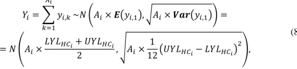
the HCi index denotes the crop that has been harvested from field i. The yield of field i (denoted with
𝑌𝑖) is the sum of the yield of each square meter within said field. Since it is assumed that the yields of
the square meters are independent and identically distributed, and the number of square meters in each field is expected to be very high, the yield of field i can be approximated with a normal distribution (in accordance with the central limit theorem) as follows:
𝑌𝑖 = ∑ 𝑦𝑖,𝑘 𝐴𝑖
𝑘=1
~𝑁 (𝐴𝑖× 𝑬(𝑦𝑖,1), √𝐴𝑖× 𝑽𝒂𝒓(𝑦𝑖,1)) =
= 𝑁 (𝐴𝑖×
𝐿𝑌𝐿𝐻𝐶𝑖+ 𝑈𝑌𝐿𝐻𝐶𝑖
2 , √𝐴𝑖× 1
12(𝑈𝑌𝐿𝐻𝐶𝑖− 𝐿𝑌𝐿𝐻𝐶𝑖) 2
),
(8)
where E is the expected value operator and Var is the variance operator. The ratio of nutrients released from crop residue is provided in Table 2. These values are also essential in calculating the total amount of nutrients returned into each field.
Table 2. Ratio of nutrients released from 1 kg of crop residue (Sebestyén, Baranyai & Boldis 1983)
Harvested Crop Returned nutrient ratio (RNR)
N P K
Wheat 0.005 0.003 0.008
Corn 0.006 0.002 0.006
Sunflower 0.008 0.003 0.001
Rape 0.004 0.002 0.005
The amount returned from nutrient j into field i is denoted with 𝑅𝑖𝑗 and equals the product of the yield of field i (denoted with 𝑌𝑖) and the returned ratio of nutrient j from the harvested crop on field i
(denoted with 𝑅𝑁𝑅𝐻𝐶𝑗 𝑖), formally:
𝑅𝑖𝑗= 𝑌𝑖× 𝑅𝑁𝑅𝐻𝐶𝑖 𝑗
, where
It is assumed that each generation of crop fully exhausts the soil, meaning that only 𝑅𝑖𝑗 is available for the next generation – the rest has to be supplied with artificial fertilizer.
The amount of nutrients required by a specific crop to achieve the national average yield varies between certain limits, as shown in Table 3.
Table 3. Nutrient amount ranges required for achieving the national average yield (eds Bocz, Késmárki, Kováts, Ruzsányi and Szabó, 1992)
Planned Crop (PC)
Nutrient requirement [kg/m2]
N P K
Lower (𝐿𝑁𝐿𝑁)
Upper (𝑈𝑁𝐿𝑁)
Lower (𝐿𝑁𝐿𝑃)
Upper (𝑈𝑁𝐿𝑃)
Lower (𝐿𝑁𝐿𝐾)
Upper (𝑈𝑁𝐿𝐾)
Wheat 0.0135 0.0135 0.0068 0.0068 0.0100 0.0100
Corn 0.0120 0.0200 0.0066 0.0204 0.0066 0.0204
Sunflower 0.0030 0.0080 0.0040 0.0120 0.0080 0.0140
Rape 0.0050 0.0110 0.0070 0.0080 0.0080 0.0100
Mathematically the amount required from nutrient j in the kth square meter of field i is a random
variable, denoted with 𝑋𝑖,𝑘𝑗 .It is assumed that the values of these random variables are independently and identically uniformly distributed between the aforementioned lower and upper limits. The lower nutrient limit from nutrient j for a square meter of field i is denoted with 𝐿𝑁𝐿𝑃𝐶
𝑖 𝑗
, where the 𝑃𝐶𝑖 index
indicates the planned crop in field i in next year’s crop rotation plan. 𝑈𝑁𝐿𝑃𝐶
𝑖 𝑗
denotes the upper nutrient limit in a similar way. Formally,
𝑋𝑖,𝑘𝑗 ~ 𝑈(𝐿𝑁𝐿𝑗𝑃𝐶𝑖, 𝑈𝑁𝐿𝑗𝑃𝐶𝑖) . (10)
The nutrient requirement of field i from nutrient j, denoted with 𝑁𝑅𝑖𝑗, can be calculated by taking the
sum of the nutrient requirement of every square meter in that field. Since it is assumed that every 𝑋𝑖,𝑘𝑗 is independent and identically distributed the central limit theorem is applicable:
𝑁𝑅𝑖𝑗 = ∑ 𝑋𝑖,𝑘𝑗
𝐴𝑖
𝑘=1
~ 𝑁 (𝐴𝑖× 𝑬(𝑋𝑖,1 𝑗
), √𝐴𝑖× 𝑽𝒂𝒓(𝑋𝑖,1 𝑗
)) =
= 𝑁 (𝐴𝑖×
𝐿𝑁𝐿𝑃𝐶𝑗 𝑖+ 𝑈𝑁𝐿𝑗𝑃𝐶𝑖
2 , √𝐴𝑖× 1
12(𝑈𝑁𝐿𝑃𝐶𝑖 𝑗
− 𝐿𝑁𝐿𝑃𝐶
𝑖 𝑗
)2) .
(11)
At this point the seed for generating scenarios is fully defined – based on these rules the second step (the simulation of scenarios) can be executed. The third step of the process is the evaluation of each scenario. To get the value of the crop residues the total expense of fertilizing with and without returning the residues to the soil has to be determined - their difference is the actual amount saved on fertilizing. To obtain the total expenses the optimization problem described in the next chapter has to be solved.
2.2. Optimization problem
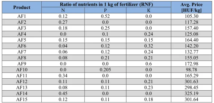
Table 4. Publicly available data of artificial fertilizer products
Product Ratio of nutrients in 1 kg of fertilizer (RNF) N Avg. Price [HUF/kg]
P K
AF1 0.12 0.52 0.0 105.30
AF2 0.27 0.0 0.0 117.28
AF3 0.18 0.25 0.0 157.40
AF4 0.0 0.1 0.24 125.08
AF5 0.15 0.15 0.15 164.40
AF6 0.04 0.12 0.32 142.20
AF7 0.06 0.12 0.24 132.77
AF8 0.08 0.21 0.21 155.05
AF9 0.0 0.0 0.6 172.98
AF10 0.0 0.205 0.0 98.78
AF11 0.34 0.0 0.0 165.29
AF12 0.11 0.11 0.21 301.63
AF13 0.08 0.11 0.23 298.45
AF14 0.45 0.0 0.0 325.19
AF15 0.12 0.11 0.18 301.64
Sources: www.agro-store.hu, www.mutragya.hu, www.gazdabolt.hu, March 3, 2015.
2.2.1. Variables
𝑋𝑖,𝑓: Real-valued variables, representing the amount of artificial fertilizer f allocated to field i in
kilograms (not to be confused with 𝑋𝑖,𝑘𝑗 , which are random variables in the simulation).
𝑌𝑖,𝑓: The binary equivalent of 𝑋𝑖,𝑓 (a flag representing whether any amount of fertilizer f is allocated to
field i – also not to be confused with 𝑌𝑖).
𝑍𝑖: The number of different types of artificial fertilizer allocated to field i. 𝑍𝑖 is calculated as
𝑍𝑖 = ∑ 𝑌𝑖,𝑓 ∀𝑓
. (12)
2.2.2. Objective function
The objective is to minimize the total expense of fertilizing. The expense of fertilizing consists of two components: the cost of artificial fertilizer and the aggregated cost of its distribution. The aggregated cost of distributing artificial fertilizer in 2014 in Hungary is 0.2889 Ft/m2 (Gockler, 2014). It is assumed that only one kind of artificial fertilizer can be distributed simultaneously on each field – therefore the aggregated cost of distributing fertilizer on a field should be multiplied by the number of different fertilizers allocated to said field. The objective function can be written as
𝑚𝑖𝑛𝑖𝑚𝑖𝑧𝑒 ∑ (∑ 𝑋𝑖,𝑓× 𝑃𝑟𝑖𝑐𝑒𝑓 ∀𝑓
+ 𝑍𝑖 × 𝐴𝑖× 0.2889) ∀𝑖
. (13)
2.2.3. Constraints
The objective is subject to only two kinds of constraints, namely to satisfy the different nutrient requirements of each field and non-negativity. The right hand side of the nutrient requirement constraints depend on whether crop residues are returned to the soil or not. Equation (13.a) shows the constraints given no residue is returned, while equation (13.b) shows the (corrected) constraints when crop residues are returned. Equation (14) is the non-negativity constraint.
∑ 𝑋𝑖,𝑓× ∀𝑓
∑ 𝑋𝑖,𝑓× ∀𝑓
𝑅𝑁𝐹𝑓𝑗 ≥ 𝑁𝑅𝑖𝑗− 𝑅𝑖𝑗, ∀𝑖, 𝑗. (14.b)
𝑋𝑖,𝑓, 𝑌𝑖,𝑓, 𝑍𝑖 ≥ 0, ∀𝑖, 𝑓. (15)
3. Simulation results
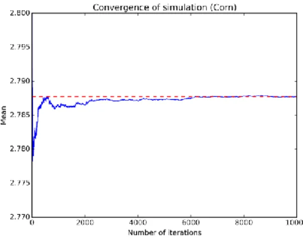
Reaching a convergent state is a key factor in case Monte Carlo simulations are involved. After 10,000 iterations the simulated results converge (Figures 1-4, convergent state represented by red dashed lines).
Figure 1. Convergence of wheat savings Figure 2. Convergence of corn savings
Figure 3. Convergence of sunflower savings Figure 4. Convergence of rape savings The expected value and standard deviation of savings are presented in Table 5. We can see that the standard deviations are very low, but considering that these values pertain only to a square meter the effects of uncertainty can vary in wide ranges given a high number of square meters involved.
Table 5. Expected value and standard deviation of savings
Residue Expected value [Ft/m2] Standard deviation [Ft/m2]
Wheat 2.4069174 0.0256387
Corn 2.7877342 0.0362423
Sunflower 0.9394069 0.0110463
Rape 4.0223666 0.1815932
Figure 5. Relative frequencies of savings on wheat residue
Figure 7. Relative frequencies of savings on sunflower residue
Figure 8. Relative frequencies of savings on rape residue
This uncertainty affects risks, thus has to be taken into consideration by financial decision making processes. Unfortunately no distributions fitted to the simulated data managed to achieve statistical significance based on the Kolmogorov-Smirnov, Anderson-Darling and 𝜒2 goodness-of-fit tests. Instead, the minimum and maximum values, the quartiles, and the 5th and 95th percentiles are provided
Table 6. Quantiles of the savings distributions
Residue Min Q0.05 Q0.25 Q0.5 Q0.75 Q0.95 Max
Wheat 2.3921173 2.3923930 2.3924884 2.3925728 2.4128814 2.4682789 2.5100094 Corn 2.7065644 2.7461959 2.7621547 2.7798875 2.8008799 2.8698510 3.0358627 Sunflower 0.9352570 0.9359759 0.9360951 0.9361143 0.9361382 0.9670020 1.0097617 Rape 3.3205631 3.6987188 3.8999960 4.0329339 4.1709930 4.2785655 4.3597880
4. Conclusions
A mathematical model has been created that utilizes Monte Carlo simulation and linear programming to obtain the distribution of savings on residues of crops grown on arable land. The model is based on general concepts and it can be used not only to determine the value of crop residues but also to optimize artificial fertilizer allocation for any number of fields with differing planned crops and residues. Although the model assumes that crops fully exhaust the soil nutrients left in the field can be included into the calculations by adding them to 𝑅𝑖𝑗. Application of this model has different positive effects as well. The permanent dosage of high amounts of artificial fertilizer sours the soil – by optimizing the required amount this process can be slowed down. The distributions of savings can also be involved in further simulations to support decision makers. It is important to note that these distributions are based on nationwide data – in different regions they might look different. Researchers or other individuals are welcome to the Python implementation of the model upon personal request or by downloading it from the journal web site.
References
Aldeseit, B. (2014) Linear Programming-Based Optimization of Synthetic Fertilizers Formulation, Journal of Agricultural Science, vol. 6, no. 12, pp. 194-201, doi: 10.5539/jas.v6n12p194
Bergez, J.E., Colbach, N., Crespo, O., Garcia, F., Jeuffroy, M.H., Justes, E., Loyce, C., Munier-Jolain, N. & Sadok, W. (2010) ‘Designing crop management systems by simulation, European Journal of Agronomy, vol. 32, no. 1, pp. 3-9, doi: 10.1016/j.eja.2009.06.001
Bocz, E., Késmárki, I., Kováts, A., Ruzsányi, L. & Szabó, M. (eds) (1992) Szántóföldi növénytermesztés (Arable farming), Mezőgazda Kiadó, Budapest
Durrett, R. (2013) Probability: Theory and Examples, 4th ed., Cambridge University Press
Fishman, G.S. (1996) Monte Carlo: Concepts, algorithms, and applications, Springer, New York
Gockler, L. (2014) A mezőgazdasági gépi munkák költsége 2014-ben (Costs of agricultural machine-related tasks in 2014), Mezőgazdasági Technika, vol. 55, no. 1, pp. 51-55.
Hansson, P-A., Svensson, S-E., Hallefält, F., Diedrichs, H. (1999) Nutrient and cost optimization of fertilizing strategies for Salix including use of organic waste products, Biomass and Bioenergy, vol. 17, no. 5, pp. 377-387, doi: 10.1016/S0961-9534(99)00050-1
King, A.J. & Wallace, S.W. (2012) Modeling with Stochastic Programming, Springer, New York
Lauwers, L., Decock, L., Dewit, J. & Wauters, E. (2010) A Monte Carlo model for simulating insufficiently remunerating risk premium: case of market failure in organic farming, International Conference on Agricultural Risk and Food Security 2010, pp. 76-89, doi: 10.1016/j.aaspro.2010.09.010
Li, X., Lu, H., He, L. & Shi, B. (2014) An inexact stochastic optimization model for agricultural irrigation management with a case study in China, Stochastic Environmental Research and Risk Assessment, vol. 28, no 2, pp. 281-295, doi: 10.1007/s00477-013-0748-4
Malcolm, D. G., Roseboom, J. H., Clark, C. E. & Fazar, W. (1959) Application of a Technique for Research and Development Program Evaluation, Operations Research, vol. 7, no. 5, pp. 646–669, doi: 10.1287/opre.7.5.646
Mínguez, M.I., Romero, C. & Domingo, J. (1988) Determining Optimum Fertilizer Combinations Through Goal Programming with Penalty Functions: An Application to Sugar Beet production in Spain, Journal of the Operational Research Society, vol. 39, no. 1, pp. 61-70, doi: 10.1057/jors.1988.8
Minh, T.T., Ranamukhaarachchi, S.L. & Jayasuriya, H.P.W. (2007) Linear Programming-Based Optimization of the Productivity and Sustainability of Crop-Livestock-Compost Manure Integrated Farming Systems in Midlands of Vietnam, ScienceAsia, vol. 33, pp. 187-195, doi: http://dx.doi.org/10.2306/scienceasia1513-1874.2007.33.187 Nábrádi, A., Pupos, T. Takácsné, Gy.K. (eds) (2007) Üzemtan II. (Agronomy II.), Debreceni Egyetem Agrár- és Műszaki Tudományok Centruma, Debrecen
Prékopa, A. 1995, Stochastic Programming, Kluwer Academic Publishers, Dordrecht
Sebestyén, E., Baranyai, F. & Boldis, O. (1983) Az őszi búza szervesanyag-termelése és tápanyagforgalma I-II (Organic matter production and nutrient turnover of winter wheat I-II), MÉM-Agroinform, Budapest
Segarra, E., Kramer, R.A. & Taylor, D.B. (1985) A stochastic programming analysis of the farm level implications of soil erosion control, Southern Journal of Agricultural Economics, vol. 17, no. 2, pp. 147-154. Vose, D. (2008) Risk Analysis: A quantitative guide, 3rd ed., John Wiley & Sons, Chichester
Winston, W.L. and Goldberg, J.B. (2004) Operations Research: Applications and algorithms, 4th ed.,
Brooks/Cole, Toronto