A comparison of two cases of low-latitude thundersnow
G. DOLIF NETO
Centro de Previsao del Tempo e Estudos Climáticos-Instituto Nacional de Pesquisas Espaciais, São Paulo, Brazil
P. S. MARKET, A. E. BECKER, B. PETTEGREW, C. MELICK, C. SCHULTZ, P. I. BUCKLEY, J. V. CLARK, A. R. LUPO
Department of Soil, Environmental and Atmospheric Sciences, University of Missouri-Columbia, MO, USA
Corresponding author: P. S. Market; e-mail: [email protected]
R. HOLLE, N. DEMETRIADES
Vaisala Incorporated, Tucson, AZ, USA
C. E. BARBIERI
Department of Parks, Recreation, and Tourism, University of Missouri-Columbia, MO, USA
Received April 16, 2008; accepted May 11, 2009
RESUMEN
Se examinan dos eventos de nevada con relámpagos en latitudes bajas a fin de identificar sus características. Ambos eventos se originaron a escala sinóptica y tuvieron impactos de pequeña escala (por ejemplo, ascenso orográfico e inestabilidad elevada). El primer evento ocurrió en el hemisferio sur y se desarrolló a finales del invierno influenciado por la orografía subyacente. Este evento presentó abundancia de relámpagos (94 destellos nube-suelo en la región); sin embargo, la acumulación de nieve fue insignificante. Este evento
fue dominado por relámpagos con polaridad negativa, con una amplitud máxima promedio de -43.2 kA.
El segundo evento fue un caso de convección elevada en el hemisferio norte con frontogénesis debajo de una capa extensa de inestabilidad potencial. Este evento también presentó abundantes relámpagos (706 destellos nube-suelo en la región), así como considerable acumulación de nieve sobre un área extensa. Este evento también fue dominado por relámpagos con polaridad negativa, con una amplitud máxima promedio
de -23.7 kA. Ambos eventos ameritan mayor investigación dado que estudios sobre tormentas similares no
son abordados frecuentemente en la literatura. Más aún, teniendo en consideración que las regiones cálidas
sub-tropicales usualmente no están preparadas para enfrentar ni siquiera los efectos de pequeñas acumula
-ciones de nieve o hielo. En el futuro, los pronosticadores pueden anticipar mejor estos eventos anómalos observando las siguientes características generales: 1) sistemas climáticos sinópticos significativos y bien definidos en bajas latitudes; 2) una zona baroclínica fuerte con estructura de chorro superpuesta bien definida
(≥60 ms-1); 3) una extensión considerable y profunda de aire frío más próximo al ecuador de lo típico; y 4)
una capa con humedad neutral a inestabilidad condicional sobre la zona frontal.
ABSTRACT
The first event occurred in the Southern Hemisphere and was a late winter case that developed under the influence of underlying orography. Lightning was plentiful in that event (94 cloud-to-ground flashes in the region), but snow accumulations were not significant. Lightning flashes of negative polarity dominated this
case, with a mean peak amplitude of -43.2 kA. The second event was a Northern Hemisphere case of eleva
-ted convection, with frontogenesis beneath an extended layer of potential instability. Appreciable lightning occurred with this event as well (706 cloud-to-ground flashes in the region), and snow accumulations were significant over a broad area. Lightning flashes of negative polarity dominated this case also, with a mean
peak amplitude of -23.7 kA. Each of these events is worthy of further scrutiny, as studies of such storms
do not appear often in the literature. Indeed, such warm, subtropical regions are often unprepared for the effects of just a little snow or ice accumulation. Future forecasters can anticipate better such anomalous events by looking for these broad features: 1) significant and well-defined synoptic-scale weather systems
at low latitudes, 2) a strong baroclinic zone with a well-defined (≥60 ms-1) jet structure aloft, 3) cold air of
appreciable depth and areal extent drawn much closer to the equator than is typical, and 4) a moist neutral to conditionally unstable layer above the frontal zone.
Keywords: Thundersnow, low-latitude, winter convection.
1. Introduction
Thundersnow can lead to deep snow accumulations and dangerous travel conditions in areas where it occurs (Crowe et al., 2006). Very often a middle-latitude occurrence (e.g. Market et al., 2002), these thundersnow storms can deposit anomalous snow totals, usually on human populations who are well-prepared to cope with their impacts (impassable roads, diminished emergency services, etc.) and return daily life to normal fairly quickly (chemical treatment of roads, physical snow removal, etc.). In short, thundersnow tends not to be a tropical or subtropical phenomenon. Yet, low latitude events do occur (e.g. Guinan 1988) -deep snow accumulations make it difficult for all, but especially problematic for those who live in areas totally unprepared for such severe winter weather. Until recently, snowstorms with lightning had received little attention in the literature; such events in lower latitudes have received even less.
The current study looks at two low-latitude snow events with lightning. One event occurred in the Southern Hemisphere in the Brazilian state of Santa Catarina. This event featured lightning and thunder during snowfall as a result of convection originating in the boundary-layer. This convection also occurred in association with a cold frontal passage and forced ascent over significant terrain; a moist neutral layer in the mid-levels was present as well. The second event considered occurred in the Northern Hemisphere over the state of Texas in the United States. This event featured lightning and thunder with elevated convection, the result of instability released above the frontal inversion well north of a surface cold front.
For these case studies, we employ a quasi-geostrophic framework for the synoptic analysis using observed data, along with output from the United States National Weather Service’s Global Forecasting System (GFS). This approach is employed to promote a more uniform, larger-scale comparison of meteorological fields between the events. On the mesoscale, comparisons are made using initial fields from the GFS as well as observed data from radiosonde flights, lightning networks, and satellite observations.
2. Case 1- Southern Hemisphere
2.1 Synopsis
On the morning of 12 September 2005, a brief thundersnow event occurred near São Joaquim, Santa Catarina, Brazil, (latitude: 28.29°S and longitude: 49.93°W). Lasting only a few minutes, the snow and thunder occurred between 1043 and 1115 UTC 12 September 2005 in São Joaquim (Cruzeiro), at an altitude of 1510 m and in the Morro da Igreja (latitude 28.12°S and longitude 49.49°W), at an altitude of 1828 m, with the surface weather station air temperature oscillating between -0.6 and +1.2°C. No measurable snowfall was reported at either station. Santa Catarina is located between latitudes 25 and 30°S, and with much of the state elevated above mean sea level by 500 m or more, snow is not unheard of there. Nevertheless, the unusual nature of this event demands further scrutiny.
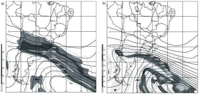
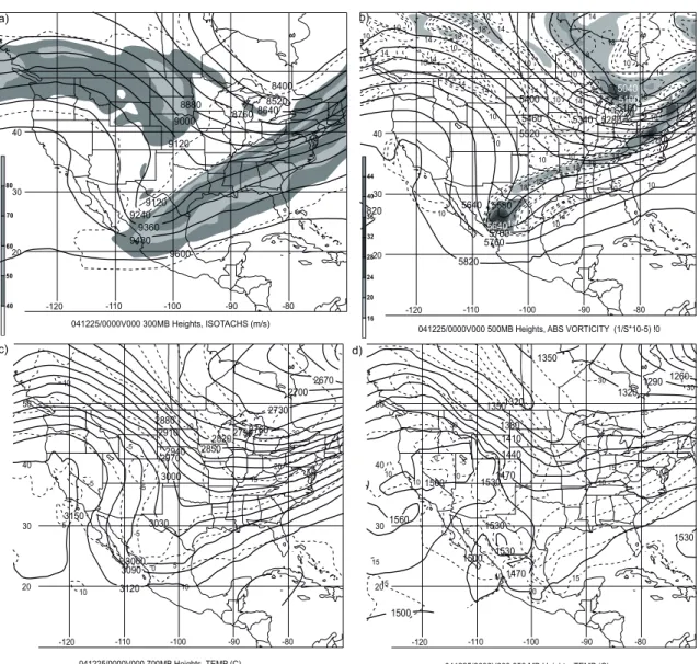
The synoptic analysis begins aloft, where at the outset the parent cyclone was an aging, occluded storm and already quite deep (952 hPa), with a surface center far southeast of the thundersnow location (Fig. 1). The thundersnow event was situated beneath the equatorward, entrance region of the 300-hPa jet streak (Fig. 2a) embedded in quasi-linear flow. Wind speeds in excess of 60 ms-1 were found to begin north of 30°S, highlighting the subtropical origins of this jet streak. This
arrangement suggests divergence aloft, and the encouragement of vertical motions over the Santa Catarina region. While across-stream ageostrophic winds and upper air divergence values were diagnosed in the appropriate quadrant at several levels (up to +6 × 10⁻⁵ s-1 at 300-hPa), they were
maximized over the state of São Paulo, some 200-250 km to the north of the event site. The 300
-hPa divergence values approached zero over Santa Catarina at 0000 UTC, but vertical motions were still robust in the lower troposphere, as the reader will see shortly.
At 500 hPa, a closed low was found near 56°S 33°W (Fig. 2b). To the north and west, elongated trough and vorticity axes were diagnosed well south of Santa Catarina, over southern Uruguay. The 500-hPa level gives a clearer picture of the age of the parent cyclone in which this event occurred. In addition to the low heights (<4980 gpm) found with the cyclone center at this level, three distinct vorticity lobes were found along and behind the leading trough. Yet, the trough axis at more northern latitudes (and thus, over the continent) was located north and downstream of the one at 300 hPa, so some baroclinic organization was still in evidence at this time. In many ways, this system resembles the cold air surges described by Lupo et al. (2001).
Fi
g.
1
. S
ou
th
A
m
er
ic
an
su
rf
ac
e a
na
ly
si
s v
al
id
at
1
20
0
U
TC
1
2
Se
pt
em
be
r 2
00
5.
S
ta
tio
n
pl
ot
s a
re
su
pp
le
m
en
te
d
w
ith
o
ut
pu
t f
ro
m
th
e G
rid
de
d
Forecast
System
(GFS)
initial
fields,
showing
sea
level
pressure
(solid,
every
4
hPa)
and
1000-500-hPa
geopotential
thickness
(dashed,
every
60
gpm).
Star
symbols
mark
the
locations
of
the
soundings
in
Figure
4,
and
the
bold,
dashed
line
represents
the
cross
sectio
n
shown
in Figure 5.
Area of interest exists between star symbols.
28
81
66
77 75
77 73 61
52 52
70 61 61
55
59 55
1
09
2
75
H
1021
59 50
5700
5580
5460
14
61
351 3
1039
55
59 55
55
H
1032
50 16
23
17 36 36 30
37
39
39
1038
H
45
45
34
34
52
52
52
52
1038
H
23
30
5580
81 72
79 68
75
82
81 75
1016
1016
H
H
73
82
2
24 172
80
82
27 150
66
82 66
26
79
2
77 61
167
73 54 72 259
69
226
77
24 203
50 50
5580
5700
1024
23
66
230
5460 5340
15
52
300 3
2
1008
5220
5340
1000
21
7
37
992 994
5220
3
84 77
270
67
5580
1026
H 102
4
55
195 6
18
64
132 3
1003
1006
5460
36
32 44
40
24
20
050912/0000v000 500 MB HEIGHTS, ABS VORTICITY (1/S*10-5) 16
28
9480
9480 9240 9360
10
10
10 10
10 10
10 4
4 10
14
14
14
14 14
5880
-70 -60 -50 -30
-30 -20 -10
-50 -40
18
-40
18
5820 5760 5700 5880
5640 5580
5520 5460
5400 5340
5280 5220
5160
5100
5040
4980
18 18
70 80
9600
50
050912/0000v000 300 MB HEIGHTS, ISOTACHS (m/s) 40
60 -40 -30 -20 -10
-50
9480
9480
9240 9360 9120
9000
8880
8760
8640
8520
-70 -60 -50 -40 -30
Fig. 2. Objective upper air analyses from the GFS initial fields for South America valid at 0000 UTC 12 September 2005: a) 300-hPa geopotential heights (solid, every 120 gpm) and isotachs (dashed, every 10
m s-1; shaded, every 10 m s-1 above 40 m s-1); b) 500-hPa geopotential heights (solid, every 60 gpm) and
absolute vorticity of the geostrophic wind (dashed every 4 × 10⁻⁵ s-1; shaded, every 4 × 10⁻⁵ s-1 above 16
× 10-5 s-1); c) 700-hPa geopotential heights (solid, every 30 gpm) and temperature (dashed, every 5°C); d)
850-hPa geopotential heights (solid, every 30 gpm) and temperature (dashed, every 5°C).
a) b)
d) c)
050912/0000V000 700 MB HEIGHTS, TEMP (C) -40
-30 -20 -10
-50
9240 9360 9120
9000
8880
8760
-70 -60 -50 -40 -30
3180
3120
5 5
5
5 5
10 10
10
10
10 10
20
3150
3120 3090 3060
3030 3000
3150
2970 2940
2910 2890
2850 2820
2790 2760
2730 2700
2670 26402610
2580
24602490 2520 3120
3090 3060
050912/0000V000 850 MB HEIGHTS, TEMP (C) -40
-30 -20 -10
-50
9240 9360 9120
-70 -60 -50 -40 -30
1530
1500
1530
20
1530
01590
1500
5
1640
5
1470
1500
10 10
1470 1440
1410 1380 1530
10
5 15
15
1560
1560
1590
1350 1320 1290
1260 1230 1200
11701140 11101180
930960 990 1020
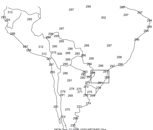
Fig. 3. A plot of surface potential temperature for various stations in South America valid at 1000 UTC 12 September 2005. Dark box approximates the region for which lightning strokes are shown in Figure 7.
2.2 Mesoscale analysis
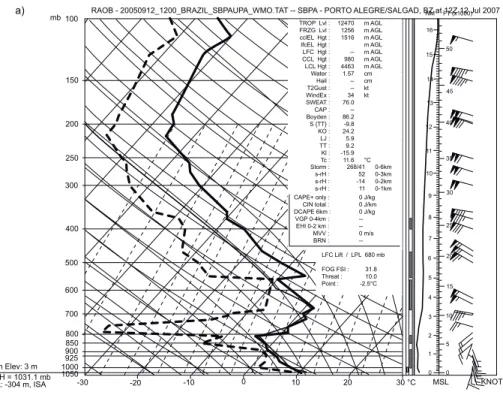
Two radiosonde ascents occurred nearby, just after the time of the thundersnow event. The first flight from Porto Alegre-Salgado Filho, Brazil (SBPA; latitude: 30.00°S and longitude: 51.18°W), was south of the surface cold front location, thus representing the cold post-frontal air (Fig. 4a). The surface layer at SBPA was nearly dry adiabatic over the lowest ~100 hPa while winds veered from southerly to westerly through the lowest ~250 hPa, marking the top of the frontal inversion layer. The second radiosonde flight (Fig. 4b) occurred in the warm air north of the cold frontal zone, from Curitiba-Afonso Peña, Brazil (SBCT; latitude: 25.52°S and longitude: 49.17°W). Although an inversion was present and based some ~50 hPa from the surface (likely the remnants of a radiation inversion), winds backed from easterly to northwesterly, suggesting a warm advection signature ahead of the cold frontal zone. A deep, nearly moist adiabatic layer occurred with this sounding, but none of the stability metrics were particularly robust; even the convective available potential energy (CAPE) for a parcel lifted from the most unstable level yielded a value of zero. Thus, the cold frontal zone and thundersnow event occurred near the time of but between these radiosonde observations, neither of which revealed significant mid-level instability. Yet, the sounding for SBPA (Fig. 4a) was conditionally unstable over the lowest ~200 hPa. Along with onshore flow (Fig. 1) and orographic lift, this sounding (Fig. 4a) suggested conditions suitable for post-frontal, low-level convection. Meanwhile the SBCT sounding (Fig. 4b), farther north and ahead of the surface cold front, revealed a deep layer that is convectively neutral.
297
297
297
297
297 297
294
294 312
312
312
299
299
298 298
289 290
295 295
295 293
293
289
288
285 267
288 288
287
287
288 288
302
209
296
296
315 308 286
290
296
290 286
285 286
281
279
281 270
274 281
278
269
271
269
275 283
281 291
280 281 280
270 274
271 275 276 273
279
274 284 281
278
RAOB - 20050912_1200_BRAZIL_SBPAUPA_WMO.TAT -- SBPA - PORTO ALEGRE/SALGAD, BZ at 12Z 12 Jul 2007
Stn Elev: 3 m
mb100 NM FT (x1000)
150
16
50 15
14
13 45
40 12
11
10
9
8
7
6
5
4
3
2
1
0 0 5 10 15 20 25 30 35 200
250
300
400
500
600
-30 -20 -10 0 10 20 30 °C MSL KNOTS
700
800 850 900 925 1000 1050 QNH = 1031.1 mb
DA: -304 m, ISA
TROP Lvl : 12470 m AGL FRZG Lvl : 1256 m AGL cclEL Hgt : 1516 m AGL lfcEL Hgt : m AGL LFC Hgt : -- m AGL CCL Hgt : 980 m AGL LCL Hgt : 4463 m AGL Water : 1.57 cm
Hail : -- cm T2Gust : -- kt WindEx : 34 kt SWEAT : 76.0
CAP : Boyden : 86.2 S {TT} : -9.8 KO : 24.2 LJ : 5.9 TT : 9.2 Kl : -15.9 Tc : 11.6 °C Storm : 268/41 0-6km s-rH : 52 0-3km s-rH : -14 0-2km s-rH : 11 0-1km CAPE+ only : 0 J/kg CIN total : 0 J/km DCAPE 6km : 0 J/kg VGP 0-4km : EHI 0-2 km : --MVV : 0 m/s BRN :
--LFC Lift / LPL 680 mb
FOG FSI : 31.8 Threat : 10.0 Point : -2.5°C
Fig. 4. Skew-T log-p plots of radiosonde data valid at 1200 UTC 12 September 2005 from a) Porto Alegre- Salgado Filho, Brazil (SBPA), which is represented by the southern star in Figure 1, south of the surface frontal zone, and b) Curitiba-Afonso Peña, Brazil (SBCT), which is indicated by the northern star in Figure 1.
a)
b) RAOB - 20050912_1200_BRAZIL_SBPAUPA_WMO.TAT -- 83840 - SBCT - ACURITIBA/ALFONSO PEN, BZ at 12Z 12 Jul 2007
mb100 NM FT (x1000)
150
16
50 15
14
13 45
40 12
11
10
9
8
7
6
5
4
3
2
1
0 0 5 10 15 20 25 30 35 200
250
300
400
500
600
-30 -20 -10 0 10 20 30 °C MSL KNOTS
700
800 850 900 925 1000 1050
TROP Lvl : -- m AGL FRZG Lvl : 3189 m AGL cclEL Hgt : 501 m AGL lfcEL Hgt : m AGL LFC Hgt : -- m AGL CCL Hgt : 307 m AGL LCL Hgt : 2455 m AGL Water : 3.21 cm
Hail : -- cm T2Gust : -- kt WindEx : -- kt SWEAT : 150.7
CAP : Boyden : 90.7 S {TT} : 26.4 KO : 15.2 LJ : 2.2 TT : 33.9 Kl : 23.6 Tc : 11.8 °C Storm : 261/25 0-6km s-rH : 259 0-3km s-rH : 99 0-2km s-rH : 0 0-1km CAPE+ only : 0 J/kg CIN total : 0 J/km DCAPE 6km : 0 J/kg VGP 0-4km : EHI 0-2 km : --MVV : 0 m/s BRN : --LFC Lift / LPL 680 mb
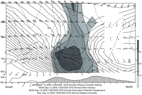
A cross section of the frontal zone (Fig. 5) revealed a well-developed baroclinic structure, with isentropes sloping down toward the warmer air, and veering winds in the lower troposphere from the warm side to the cold side of the front (cold southerlies south of the front and warm northerlies to the north of the frontal zone). The frontal zone intersected the surface of the earth (in a region where the terrain extends as high as ~900 hPa) near the center of this analysis (Fig. 5). A jet structure was present at 300 hPa with speeds in excess of 100 kt, aloft and poleward of the surface frontal location. In addition, a direct thermal circulation was suggested in the thinned (grid spacing of 2.5° latitude
× 2.5° longitude) GFS fields, with ascent (<-3 μb s-1) embedded in a nearly-saturated region of the
mid-troposphere just poleward of the surface frontal zone. Farther south, a region of descent (>3 μb s-1) was found just above the frontal zone and beneath the upper level jet streak. Finally, note that the
best moisture and ascent not only occurred near the location of the surface frontal zone, but above a region of significant terrain and with a shallow layer of elevated potential instability.
Fig. 5. Cross-section from the GFS initial fields for South America valid at 1200 UTC 12 September 2005 along the line shown in Figure 1. Winds are plotted in station model format (in knots), with relative humidity (shaded every 10% above 70%), equivalent potential temperature (solid, every 2 K), and pressure vertical
velocity (dashed, every 1 μb s-1).
Satellite imagery (Fig. 6) showed the coldest over-land temperatures were found over the western reaches of Santa Catarina, with onshore cloud top temperatures generally warmer than
-40°C. Nevertheless, the analysis of cloud-to-ground lightning flashes (Fig. 7) revealed a steady northward progression of the flash patterns that attended the motion of the frontal zone, with numerous flashes detected over Santa Catarina and Paraná during the period in question. Lightning flash frequency was never very high with this system, and was also on the decline between 0800 and 1100 UTC over the state of Santa Catarina. There were 47 cloud-to-ground lightning flashes over the entire state between 0800 and 0900 UTC, 27 between 0900 and 1000 UTC, but only 20 flashes between 1000 and 1100 UTC (the time period of interest) for the same area. Interestingly, no flashes occurred in the area after 1100 UTC, so we speculate that reports of thunder by human
300
3 400
500
700
850
925
1000 South
320 324
70 70
328 336
328 316
308 304 300 296 292
288 312
332
324
90
80
70
North MON SEP 12 2005 1200V000 GFS thinned Pressure Vertical Velocity
MON Sep 12 2005 1200V000 GFS thinned Wind Vectors MON Sep 12 2005 1200V000 GFS thinned Equivalent Potential Temperature
observers as late as 1115 UTC may well have been borne of in-cloud lightning flashes. Of the 94 cloud-to-ground flashes, 79 (84%) were of negative polarity and 15 (16%) were of positive polarity. Negative flashes had a mean peak amplitude of -43.2 kA (±33.6 kA); the median peak amplitude was -29 kA. Positive flashes had a mean peak amplitude of +38.1 kA (±17.5 kA); the median peak amplitude was +37 kA. The relatively widespread nature of these lightning flashes suggests that thundersnow may have been experienced more widely than was reported. However, that conclusion must also be tempered by the notion that the stations reporting thundersnow were at a relatively high altitude.
Fig. 6. GOES-12 infrared satellite image of South America from 1030 UTC 12 September 2005. The temperature scale °C is show at bottom right.
Fig. 7. Lightning strokes from the Brazilian Lightning Detection Network (BrasilDat) for the 3-hour period 0800 to 1100 UTC 12 September 2005. Color coding breaks flashes into 1-hour subperiods.
20050912 1030z
(graus Celsius)
-30 -40 -50 -60 -70
Porto Alegre RS
PR
S. Joaquim
M. Igreja Florianopolis
Morianopolis Cuchilla
Sao Joaquim (Cruzeiro)
25S
Morro da Igreja
Florianopoli
s
25.5S
26S
26.5S
27S
27.5S
28S
28.5S
29S
29.5S
30S
55W 54.5W 54W 53.5W 53W 52.5W 52W 51.5W 51W
8 9 10 11
50.5W 50W 49.5W 49W 48.5W 48W
3. Case 2 – Northern Hemisphere
3.1 Synopsis
Thundersnow occurred along the Gulf of México coast of the state of Texas in the United States late in the day of 24 December 2004. Situated between 24 and 29°N latitude, snow totals of 31.8 cm and 11.2 cm were measured at Victoria, Texas, and Corpus Christi, Texas, respectively. Even Brownsville, Texas, on the US-México border measured 3.8 cm of snow. The thundersnow event that developed late on 24 December 2004 across southern Texas occurred in the wake of a previous cold frontal passage (Fig. 8); this surface frontal zone was supported by a significant long wave pattern in the mid- to upper-troposphere and a surge of cold air in the lower troposphere. By 0000 UTC 25 December 2004, a closed low had appeared over the Big Bend region of Texas at the 300-hPa level, with the Texas coast found beneath the axis of the subtropical jet (Fig. 9a). Indeed, the 300-hPa low and associated short wave trough lagged behind the larger longwave system, whose center at this time was far to the north over the Hudson Bay area. The development of the closed low was partially a response to the deep column of cold air that had become concentrated beneath the upper low, which will be discussed at greater length shortly. At 500-hPa (Fig. 9b), a distinct circulation was present in the vorticity field over the northern third of México, although a closed low was not present at this level. Cyclonic vorticity advection by the geostrophic wind was indicated downstream of the trough axis, although the signature was weak over coastal Texas. Of interest, too is the band of shear vorticity across the southern and eastern United States that served as a testament to the history of this system and the greater phase speed of the northern wave which, until recently, had been a part of the much larger long wave pattern.
Fig. 8. United States Hydrometeorological Prediction Center surface analysis valid at 0000 UTC 25 December 2004. Star symbol marks the location of the soundings in Figure 10, and the bold, dashed line represents the cross section shown in Figure 11.
8 9 43 244 270708 200506 VRWQ230 8 9 9 46004 42 161 11207 46 220
45 18070546036 DEHY43 200604 +15 +1 +1 19 +30 0 0 0 46 183
1020-19205
46005 12 53 214 CGQD343 46651 11 -28 -24 11205001204 52
3ERW249 220 -10 20601 15 38 251202 235 -3 37 -25 218 43 42 K53S0 4 CG 9584 45 45 207 4614 473 43 250406 112 32 34 105 130 40 10200 55 116 152 25 21 173 34 1001 1016 30 150 132 41 177 20 27 28 37 042 040 047 -6 -18 10 -22 -13 -26 10 -31 144-35 -38 -45 -35243 253 225 163 1 107 -44 -18 -18 -11 -17 -13 -26 -44 -33 -6 10 074 9 13 27 37 26 124 38 38 178 40 109 21 38 132 24 31 168 25 21 223 28 20731
17 32 197 21 170 27 12 27 19011 15 0
24 26
19 0 3 0 24280960 928 14
15 101 14 -1 18 23 -2 34 135 35 20 21
27 15 10
21 184 199 15 233-4
262 -8 2 18 -1 20 216
255 0
1029 1028 1028 5 231 5 20 24 220 9 16 19 12 211
23 25 23323 235 12 14
25 260
15 18
28 255 21
16 -15 5 280 273 27 268 19 279 9 5 25 17 16 29 15 32 231 33
21 33 240 2352436 49
35 22 0 201 042 0 17 15 13 256 35 277 35 12 35 34 28 220 8
67 145 10704 1012 125 o 201 010800
-90120 -85 -80
82 125 75 131 79 125 100502 -75 29 26 ZCBU274 000000 20401 77 133
79 ZCDG869 77 79 HBNE73 20302 79 72 28 010802 27 27 26 4200358 10504 66 61 5055 52 42 0
153 SPGP17370 C6FN568 20402 120 75 130804 7575 0 51 24 176 00090123 4100960 691060 162 62 71143
20403 TNF135
216 28 0
210 37 3820140 188
28 23 36 27 19
248248 40 26 229 23
272 12 21 25115
14 23
33 271 236 17 200 34 19 36 21 278 -8
23 249 18 12 30 215 3440 331 213 192 10804 205 140 71 4100261 213
19 30 178 193 WPV06324
050803 70 125 219 35 CLKN745 19 34401436 10804
180 00090210903 207 15 000905 70 200 090905 20301 PFRX62 63 68 211 70 PFASG48200402 21 22 218 22 092 19 29 240 43 12 12 0 271 8 10 22 160
0 2410 12 227
15 216 309 131003 10906
204
4400438 15
242 1 244 246 ** LSCM14
5
215 23 2052 11003 47 174 8 14 00100210806VRXL646
52 10906 110 140 41 4401 11003 192 11 30 9 186 172 4400829 32 198 2109 30 44005
26 200 182 VD7857 0 18 11 200 21 16 226 10YGR 14 1 1 196BANG1 212
9 -11** **
-4206 **-2 -27 222
-22 -33
-22 225 -17 -13 -15 -11 215 215 230
B -2 10 9 4460716 10806 127 118
9 212 0 27 12129
6 5 8
-9 9 -2
1871025 23 18612
21 088 63 37 36
101 127
34 CG2994H 441 39
48 57 250 41623 55 186 10805 SKWI V78M5528 222 12 160 41 5 50 15 142 44137 51 h125 -5 149 30 28151 30 9 144161
0 10301 126 30 32 32 401 1016 5 19712 44035 205
121020 1 225-29
-18
o
1 222-2 -9215-6 14 19321
3 12 44002520 39 213 211 37 13 39 19 FPSN7 22 10804 410044135 39 22 213 37 1013 1012 1018 193 234 40 213 410084226 16 10702000701
0 41 49 157 13943 26 76 73 147 VENF152 66 6868 146
24 1 132SMK=168 155 21 180 52 180 196 420394710502 10602
68 WABU66 20402 28 26 75 79 79 72 75 72 75 70 68 75 79146 ELWX571 MCZN274 112 79 75 140 14 48 200 LUML126 10502 21 56 70 164 4204151 1060423
050805 V2AJ170 24 76 205044200162 20608 360506 22 CGYE45 226 35 25503529 265 11 025
32 144 PTAT225 16 34 16 30 246244 18 31 260 21 18 25228 31 259 14
32 15 0
32 25 271 12
12 28 29 270 16 21 243 250 13 9 19 247 0 25 26 15 247 277 14 12 14 37 248 15
249 13 30 14 34 14 256 262 12 36 34 27 34 251 260
34 28 50 62 -100 -105 52 -95 45 178 = = 29 32 219 4200260 24 24 64 13820
WCX533362 10907 0 36 27 1008 1003 1003 34 25 0 1917 28 123 138 4 054 -9 -2 -27-2 -22-27
0 -6 -18
-11 -17 -13
SGNW3221 -9 224 251 279 13 2 20 14 -13 -7 12 214 1 205 -8 -15 -7 10 198 -6 4 23 -3 -6 236 -5 -1 7 0 1 -9 -4 226 -15
-5 22 315198 193 -24
1020
1005
1019
215
-29 -17-26215 -35 -6 133 DISW3 228 -4 0 7 5 -22 -17 -42 -26 -33 236 199 135 088 086 114 -13 7 7 7 -7 0 1 16 9 17 21 0853 112
0 6 6 0 3 -13 -8 4 0 0 068 3 -38 -36
-36 -9 146
-17 -18 177
-13 22 149 1012 + ** ** ** ** ** ** ** ** -26 -22 -31 243 -18 -31243 -40 261 445 25 -27 127 063 136 238 188 -8 -15 093 7 071 146 32 25 34 32 231 1008 1004 37 34 30 41 19 20204 23 229 237 -20 -8 -1 +5 +3 +5
+3 -4 +10
+8
+9 +13
+5
+11 +8 -8 -9
-18 -17 -14 -15 -2 +10 -4 -17 -21 -10 +7 +9 -5 -10 -6
-5 -7 -7
-11 -8 +2 -3 5 +7 -3 +2 -20 0 +9 +5 -15 0 0
-60 -14 0
-1 0 +12 -1 +9 -4 -1 +2 0 -3 -7 +3 +1 +5 +12
+10 +6 +6 +4 0 0 0 +12 +20 -12 +14 +10 -30 -20 -4 -20 +18 +7 -8 +11 -5 +17 +15 +6 -6 -3 -6 +3 +11 +13 +7 +4 -8 -5 +2 +10
+5 +12 +5
+21 +16 +21 +22 +2 +16 0 -5 -7 +3 +4 0 0 9 0 +12 +10 -5 -10 +7 16 -4 0 -21 -24 -17 -9 -6 -2 -7 +7 -7 -9 -19 -17 -28 -26 -21 -20 -14 -6 -17 -13 -9 -8 -12 -13 -6 -3 -7 -12 +5 +11 -1 -1 0 +10 +1 0 39 216
32 235 28 -16 27 170 18 247 37 28 070 39 30 37 029 14 055 34 27 28
104 08634 23 40 27 23 37 053 053 057 041 08028 36 34 34 25 25 -1730 = 241 30
-20 -21 -17 25 238 33 27 1032 1024 47 227 -20 -20 32 25 41 28 37 122 1829 29 37 289 32= -2240 212
-24 -20 49
34 52 236
275 10 1 26 42 22 2748 40 19 32 -19 -29 -19 272 11305 40 46002 13 51 258 11404 258 46652 56 14 258 -12 11405 46059 15 3 280 60 260 57 17 20000 -30 -20 354
260 15 030802 20301
250 58 02080 14480
6--20301 ELWR551 14 20100
341206 58 238 WRYW46 12 46013 13 -2 4604213 0 27 25 19 232 147 32 295 31 24 4601510 52 49 56 NWP0344
11704-5 242 27-21 42 244 -2 25 272 -20 -16 -16 -16 -18 41 19 296 59 30 252 19 350603 MKYJ851820000 -30 -2 -10 -10 -10 -3 -2 -10 -1 +1 -3 -3 -7 -1 +4 -20 -7 -4 +2 +4 +5 +1 -15 -8 -11 -7 -5 9 23344 237 265 18 44 563524648 -16 -13 -9 -14 -13 -11 -7 -3 -2 -10 -14 -1 -3 -3 +3 -3 +3 40 11604 001604257 56 56-8
-13 37 57 50 61 46054 48 57 37 14 281603160350 46047 34 11603 17 60 H H H H H H L L L L 7 27 234 5 52 2 225 1032 1032 1028
35 276 25 4 251 272 4 28 1034 1002 1024 1012 0 226 239 61 64 63 2311001 234 11 12 1 264 6 34 22 315 27 0 286 17 11703 240 55 25039 25039 15 15
257 50 237 45 16 30 323 15 300 37 37 30 3 6 26 3
20 3040 21 266 25 22230 12 21 18 15 14 279 1 45 025 25 31 307 296 16 6 301 62 2114414
259 15 34 304 14 21 19 284 257 11603 K3L3 239 001603 16 66 250 65 231 -17 36 -3 -13 -15 60 25
DHKW51 203023603020 0
75 -10
-30
-120 -115 -110
ZCDF849 24 66 37 100 68 166 46 66 43 64 179 48 360603 153 64 30 23 70 41 45 59 123 34 30 1001 DIHE40 17 62 45 192 6 43 41 42
230 30
211 8
8 3323419
15 23 63 68 54 63 225 L L L
5820 40
30
20
-120 -110 -100 -90 -80
44
36
28
24
16
041225/0000V000 500MB Heights, ABS VORTICITY (1/S*10-5) !0
20 32 40
57605700
5640
5580 10
10 10
14 14
14 10 14 14 14
10 10
10 10 14 18 18
10 14
10
10 10
14 18 18
18
18 18 10 5520
5460 5400 10 14
5340
5040
10
14 14
18 18
10
5100
5160 5220 528010
10 10
10 10 18
14
5640 5820
18
8880
8400 8520 8640 8760 9000
9120
9120 9240
9360 9480
9600
40
30
20
-120 -110 -100 -90 -80
80
70
60
50
40
041225/0000V000 300MB Heights, ISOTACHS (m/s)
In the lower troposphere, the cold-core signature of this cyclone became more clear with the broad shortwave trough at 700-hPa (Fig. 9c) beneath the ones found at 300 and 500-hPa and the coldest air found along 700-hPa trough axis. To the east over the Texas Gulf coast, only the southernmost tip of the state was above freezing at this level, but a broad thermal gradient was also observed along and parallel to the coastline. A similar thermal pattern was found along the Texas Gulf coast at 850-hPa (Fig. 9d), with the 0°C isotherm immediately along the coastline. At the surface (Fig. 8), a broad region of high pressure was positioned across northern Texas and northeastern México. The cold front that had moved through south Texas previously was analyzed at this time as a stationary front well south into the Gulf of México. An inverted trough was oriented perpendicular to the Texas Gulf coast in the vicinity of Corpus Christi, where near-freezing temperatures, wintry precipitation, and a moderate northerly breeze were observed.
Fig. 9. As in Figure 2, but valid over North America at 0000 UTC 25 December 2004. b)
a)
c) d)
-120 20
-110 -100 -90 -80
041225/0000V000 700MB Heights, TEMP (C) 3150
10
10 5
30 40 50
5
5 -5 -5
-5 -10
-30
10
-20 15 2880
2910 2940 2970 3000
3030
3060 3090 3120
0
285028202790 2760
2730 2700 2670
-120 20
-110 -100 -90 -80
041225/0000V000 850 MB Heights, TEMP (C)
15
30 40 50
1500
1470 1500 1530
1530 15301470
1560 1500
1440 1410 1380 13501320
1350
13201290 1260
1530
15 15
10
10 10
0 5
30
30
10 15 -5
30
5 10
20 15
3.2 Mesoscale analysis
Cold, post-frontal air was present in the lowest ~250 hPa of the sounding from Corpus Christi, Texas (KCRP; latitude: 27.77°N and longitude: 97.50°W), flown at 0000 UTC 25 December 2004 (Fig. 10). Indeed, surface winds were northerly, becoming easterly with height and finally switching to a more southerly flow at and above the frontal inversion, demonstrating a clear profile of veering with height. While this would usually suggest the presence of warm advection (WAD) in the layer, diagnostics at 850 hPa failed to show a significant region of WAD at that level. Yet, the sounding revealed significant mid-tropospheric instability above the frontal inversion (Fig. 10). The 700-500-hPa lapse rate value of 7.3 K km-1 translated into a Lifted Index of -13 and a CAPE
of 155 J kg-1, both for a parcel originating at 700 hPa; these values are in line with those found
by Market (2006) for central US thundersnow events. This plot suggests a region that approached the criteria for a moist absolutely unstable layer (e. g. Bryan and Fritsch, 2000) and conducive to the development of upright convection.
Fig. 10. Skew-T log-p plots of radiosonde data valid at 0000 UTC 25 December 2004 from Corpus Christi, Texas, United States, which is represented by the star in Figure 8.
RAOB - 20041225_0000_TEXAS_KCRPUPA_WMO.TXT -- 72251 - KCRP CORPUS CHI
Stn Elev: 13 m
mb100 NM FT (x1000)
150
16
50 15
14
13 45
40 12
11
10
9
8
7
6
5
4
3
2
1
0 0
5 10 15 20 25 30 35
200
250
300
400
500
600
-30
-40 -20 -10 0 10 20 30 °C MSL KNOTS 700
800 850 900 925 1000 1050 QNH = 1023.3 mb DA: -598 m, ISA
TROP Lvl : 13508 m AGL FRZG Lvl : 116 m AGL cclEL Hgt : 5330 m AGL lfcEL Hgt : 7196 m AGL LFC Hgt : 3854 m AGL CCL Hgt : 5253 m AGL LCL Hgt : 3117 m AGL Water : 1.74 cm
Hail : ---- cm T2Gust : -- kt WindEx : 11 kt SWEAT : 97.0
CAP : 0.3 Boyden : 84.1 S {TT} : 27.9 KO : 28.2 LJ : -1.3 TT : 34.7 Kl : 15.4 Tc : 37.7 °C Storm : 266/29 0-6km s-rH : 732 0-3km s-rH : 268 0-2km s-rH : 42 0-1km CAPE+ only : 155 J/kg CAPE 0-3km: 0 J/kg CIN total : -4 J/km DCAPE 6km : 1059 J/kg VGP 0-4km : 0.2 EHI 0-2 km : 3
MVV : 18 m/s
BRN : 1
LFC Lift / LPL 700 mb
FOG FSI : 36.8 Threat : 7.5 Point : 4.2°C
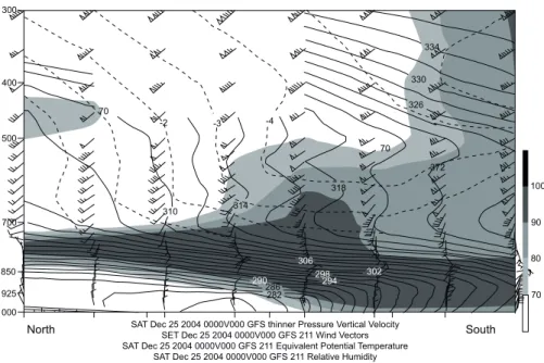
Cross section analysis (Fig. 11) revealed the presence of potential instability over a broad region above the frontal inversion. Moreover, this layer resided south of and above a region of mid-level frontogenesis (>1.0 K 100 km-1 3 h-1), where the upward vertical motions were already in excess
of 5 μb s-1. However, it is important to note that the occurrence of thundersnow went on well
Fig. 11. Cross section from the GFS initial fields for the Texas Gulf coast valid at 0000 UTC 25 December 2004 along the line shown in Figure 8. Winds are plotted in station model format (in knots), with relative humidity (shaded every 10% above 70%), equivalent potential temperature (solid, every 2 K), and pressure
vertical velocity (dashed, every 1 μb s-1).
300
70 400
500
700
850
SAT Dec 25 2004 0000V000 GFS thinner Pressure Vertical Velocity SET Dec 25 2004 0000V000 GFS 211 Wind Vectors SAT Dec 25 2004 0000V000 GFS 211 Equivalent Potential Temperature
SAT Dec 25 2004 0000V000 GFS 211 Relative Humidity 925
1000
North South
-2 -3 -4
310 314
290 306
298294 286
282
302 318
70
100 372
326 330
334
90
80
70
The satellite imagery appeared deceptively benign with the coldest cloud tops, associated with the larger cloud mass, found well off the Texas coast (Fig.12). Small nascent cloud bands were beginning to emerge over southern Texas with cloud top temperatures of ~ -40°C. Banding was present in the precipitation field, as rendered by radar (not shown), and lightning activity (as revealed by the North American Lightning Detection Network) attended these bands, the full history of which is shown in Figure 13. This event occurred over a much longer time period, so data for a full 24-hour period are supplied. Of the 706 cloud-to-ground flashes shown over the 24-hour period, 511 (72%) were of negative polarity, and 195 (28%) were positive. However, only 16 of the flashes shown in Figure 13 occurred onshore during this time. Therefore, the flash density and frequency were quite low for those onshore flashes that occurred primarily with snowfall. No real trend was apparent in the onshore flashes, although the period of peak activity was clearly between 1800 UTC 24 December 2004 and 0000 UTC 25 December 2004 (the blue dots). Of the 16 flashes that occurred well onshore, only one was positive and had a peak amplitude of +45.4 kA. The remaining 15 cloud-to-ground flashes that occurred well onshore had a mean peak amplitude of
-24.2 kA (±17.2 kA); the median value was -17.2 kA. Being deeper into the cold season than the Southern Hemisphere case, it comes as no surprise that both the flash density and the flash frequency are lower with this event.
Fig. 12. GOES-12 infrared satellite image 2345 UTC 25 December 2004. The color table is used to denote the temperature scale, shown at left.
Fig. 13. Cloud-to-ground flashes from the North American Lightning Detection Network for the 24-hour period 1200 UTC 24 December to 1200 UTC 25 December 2004.
Color coding breaks flashes into 6-hour subperiods.
profile are all in line with the experimental findings of Takahashi (1978) as well as later field investigations (Takahashi et al., 1999). Specifically, this thermodynamic profile allowed for a positively buoyant parcel through a deep layer. Also, such a convective cloud would cross over both the -10°C level (a known charge reversal temperature) and -20°C, a level known for active particle charging processes (provided adequate moisture; Takahashi et al., 1999).
4. Summary
Two cases of thundersnow are examined from the low latitude regions of both the Northern and Southern Hemispheres. The event over southern Brazil was marked by onshore and upslope flow near the surface, while the Texas coast event had no comparable topographic relief, and an offshore surface flow regime. The idea that terrain played a role in the Brazilian event is supported by the
nearby soundings, both of which originate from close to sea level. Indeed, the post-frontal sounding
from SBPA (Fig. 4a) is cold enough to support snowfall down to 1510 m MSL (and below), yet above, the profile is roughly isothermal about freezing up to ~700 hPa. Moreover, the surface
conditions evince an atmosphere that is quite unstable, suggesting that surface-based convection
was likely. In conjunction with the other regional sounding (Fig. 4b), the Brazilian case appears to have been one of forced ascent over orography, with snow falling from a larger, parent stratiform cloud but with embedded convection.
The event over the Texas coast resulted from the release of elevated instability. It is true that the near-surface flow was offshore, and topographic relief of the kind in the Brazilian case does not exist in coastal Texas. Moreover, the Brazilian case had the benefit of a frontal zone in the immediate area, having passed through the region with thundersnow only hours prior. By contrast, the Texas thundersnow occurred north of a cold frontal zone that had moved through two days prior. More importantly, the thundersnow represented the release of elevated potential instability above the frontal zone.
To summarize, both of the cases were the product of significant and well-defined synoptic-scale weather systems at low latitudes. A strong baroclinic zone was also present in both cases, with a well-defined upper-tropospheric jet structure aloft in support of a lower-tropospheric front. In each case, cold air of appreciable depth and areal extent was drawn much closer to the equator than is typical. Yet, important distinctions existed between these cases on the smaller scale. In both events, a moist neutral thermal profile existed in the mid-troposphere, but external, low-level forcing for ascent was of much greater importance in the Southern Hemisphere event. That forecasters at low latitudes (and lower altitudes) find themselves in a situation where snow is likely or already occurring clearly indicates an anomalous event. It is not unreasonable, then, that such events may also possess dynamics sufficient to create heavy snowfall, and perhaps thundersnow.
Should the synoptic and mesoscale situation appear conducive to snowfall, then one may also assess the likelihood of thundersnow. On the larger scale, forecasters can anticipate such anomalous snow events by looking for these features: 1) significant and well-defined synoptic-scale weather systems at low latitudes, 2) a strong baroclinic zone with a well-defined (≥60 ms-1) jet structure
(especially in the absence of orography), 3) have the most unstable parcel originate from a level where the temperature is warmer than -10°C, and 4) have the equilibrium level of the parcel in number 3 above extend to a level where the temperature is colder than -20°C.
Acknowledgements
The authors would like to thank the two anonymous reviewers whose efforts produced an improved manuscript. This work is supported by the National Science Foundation (NSF), Award No. ATM
-0239010. Any opinions, findings, conclusions or recommendations expressed herein are those of the authors and do not necessarily reflect the views of the NSF.
References
Bryan G. H. and M. J. Fritsch, 2000. Moist absolute instability: The sixth static stability state. Bull.
Amer. Meteor. Soc. 81, 1207-1230.
Crowe C. C., P. S. Market, B. P. Pettegrew, C. J. Melick and J. Podzimek, 2006. An investiga -tion of thundersnow and deep snow accumula-tions. Geophys. Res. Lett. 33, L24812, doi: 10.1029/2006GL028214.
Guinan P. E., 1988. A case study of an intense south Texas snowstorm during January 12-13, 1985. M. S. Thesis, University of Illinois at Urbana-Champaign, 103 pp.
Lupo A. R., J. J. Nocera, L. F. Bosart, E. G. Hoffman and D. J. Knight, 2001. South American cold surges: Types, composites and case studies. Mon. Wea. Rev.129, 1021-1041.
Market P. S., C. E. Halcomb and R. L. Ebert, 2002. A climatology of thundersnow events over the contiguous United States. Wea. Forecast.17, 1290-1295.
Market P. S., A. M. Oravetz, D. Gaede, E. Bookbinder, A. R. Lupo, C. J. Melick, L. L. Smith, R. Thomas, R. Redburn, B. P. Pettegrew and A. E. Becker, 2006. Proximity soundings of thunders -now in the central United States. J. Geophys. Res. 111, D19208, doi:10.1029/2006JD007061. Morales R. F., 2008. The historic christmas 2004 south Texas snow event: Diagnosis of the heavy
snow band. Nat. Wea. Dig. 32, 135-152.
Takahashi T., 1978. Riming electrification as a charge generation mechanism in thunderstorms. J.
Atmos. Sci.35, 1536-1548.