Principled Approaches to Missing Data in Epidemiologic Studies
Neil J. Perkins, Stephen R. Cole, Ofer Harel, Eric J. Tchetgen Tchetgen, BaoLuo Sun, Emily M. Mitchell, and Enrique F. Schisterman*
*Correspondence to Dr. Enrique F. Schisterman, Epidemiology Branch, Division of Intramural Population Health Research, Eunice
Kennedy Shriver National Institute of Child Health and Human Development, 6710B Rockledge Drive, Room 3136, MSC 7004, Bethesda, MD 20817 (e-mail: [email protected]).
Initially submitted May 19, 2016; accepted for publication September 12, 2017.
Principled methods with which to appropriately analyze missing data have long existed; however, broad implemen-tation of these methods remains challenging. In this and 2 companion papers (Am J Epidemiol.2018;187(3):576– 584 andAm J Epidemiol.2018;187(3):585–591), we discuss issues pertaining to missing data in the epidemiologic literature. We provide details regarding missing-data mechanisms and nomenclature and encourage the conduct of principled analyses through a detailed comparison of multiple imputation and inverse probability weighting. Data from the Collaborative Perinatal Project, a multisite US study conducted from 1959 to 1974, are used to create a masked data-analytical challenge with missing data induced by known mechanisms. We illustrate the deleterious effects of missing data with naive methods and show how principled methods can sometimes mitigate such effects. For exam-ple, when data were missing at random, naive methods showed a spurious protective effect of smoking on the risk of spontaneous abortion (odds ratio (OR)=0.43, 95% confidence interval (CI): 0.19, 0.93), while implementation of prin-cipled methods multiple imputation (OR=1.30, 95% CI: 0.95, 1.77) or augmented inverse probability weighting (OR=1.40, 95% CI: 1.00, 1.97) provided estimates closer to the“true”full-data effect (OR=1.31, 95% CI: 1.05, 1.64). We call for greater acknowledgement of and attention to missing data and for the broad use of principled missing-data methods in epidemiologic research.
bias (epidemiology); complete-case analysis; inverse probability weighting; missing data; multiple imputation
Abbreviations: BMI, body mass index; CPP, Collaborative Perinatal Project; IPW, inverse probability weighting; MAR, missing at random; MCAR, missing completely at random; MI, multiple imputation; MNAR, missing not at random.
Missing data are a pervasive challenge in biomedical research (1). For example, of 262 studies published in the 2010 volumes of theAmerican Journal of Epidemiology,Epidemiology, and the International Journal of Epidemiology, the amount of missing data was not sufficiently reported to be quantified by reviewers in 68% (2). When quantifiable, the extent of missing data can be substantial. For example, Eekhout et al. (2) re-ported a prevalence of 26% missing data in 84 epidemiologic studies. Although missing data are nearly ubiquitous in epi-demiologic research, the impact of missing data on inference can vary greatly.
Despite a rich body of literature on statistical methods for the analysis of missing data, the most widely used technique in epidemiology remains the most basic:“complete-case” analysis (2–10), which ignores potentially valuable observed
information by excluding participants with only partially available data on the variables of interest (11,12).
To demonstrate the impact of missing data and illustrate prin-cipled methods that account for missingness, we constructed a challenge with 2 independent teams of missing-data experts. The goal of their work was to illustrate the use of methods of their choice to analyze epidemiologic studies with missing data and to evaluate and relax (to the extent possible) the assump-tions made about missing data.
MNAR cannot be ruled out empirically and typically implies that aspects of the missing-data mechanism need to be properly modeled to identify the parameter of interest. Intuitively, the observed data are of little help, because the information neces-sary to model the missing-data mechanism is unobserved by definition (18,19). Therefore, modeling missing data that are MNAR often requires additional assumptions either in the form of external information or fairly strong parametric as-sumptions when such information is not available (20,21). Other approaches to handling MNAR data include conducting a sensitivity analysis, which in extreme scenarios will produce bounds for the impact of missing data. If data are MNAR, then both complete-case analysis and the principled methods dis-cussed in the companion papers may provide biased estimates. Notably, MNAR does not imply or guarantee biased estimates, which depends on the particular causal structure; it only guaran-tees that we cannot correct for it if present (22).
Finally, ignorability is a criterion that is often used inter-changeably with MAR but requires that the missing data are MAR (or MCAR) and that the parameters governing the missing-data mechanism are distinct from the parameters governing the full-data model (16,23). Little and Zanganeh (24) have provided a variety of examples where a data set is MNAR and how ignorability can arise and be used in a subset to perform valid inference on that subset of data. Distinct param-eters are those for which, in the likelihood setting, the domain of the parameters is the Cartesian product of their individual do-mains (values taken by one parameter do not restrict values taken by another parameter); and in the Bayesian setting, distinct parameters require independent priors for the param-eters. Ignorability (e.g., MAR with distinct parameters) is the weakest general assumption that allows the likelihood to factor such that one can identify the parameter of interest. In set-tings where ignorability does not appear to hold, methods for nonignorable models (e.g., pattern mixture models) can be useful (25).
MOTIVATING EXAMPLE
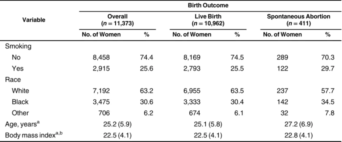
Data for this challenge comprised information on a subsample of participants from the CPP. The CPP was a multisite US study of pregnancy and pediatric outcomes conducted from 1959 to 1974 (13). The CPP investigators recruited and enrolled 48,197 participants who were seeking prenatal care. Data on demographic factors and medical history were collected at entry into the study. For illustrative purposes, we selected 11,373 women entering the cohort prior to 20 weeks’gestation who had complete data on the variables birth outcome (spontaneous abortion (<20 weeks’ ges-tation) or live birth), maternal smoking, maternal age (years), maternal race, and maternal body mass index (BMI; weight (kg)/ height (m)2). Spontaneous abortion or live birth and smoking sta-tus were binary variables; race was categorized as white, black, or other; and age and BMI were continuous. This subsample is referred to as the“full”data set. The characteristics of the full data set are displayed in Table1, overall and by birth out-come, with 411 spontaneous abortions and 10,962 live births.
The missing-data analytical teams were asked to estimate the relationship between smoking exposure measured dur-ing early pregnancy and the risk of spontaneous abortion differentmechanisms.Twoteamsthenanalyzedtheexample
datasets,oneusingmultipleimputation(MI)toaccountfor themissingdata(14)andtheotherusinginverseprobability weighting(IPW)(15).Whileinpracticeresearchersmayhave substantiveinformationregarding themissingnessprocess, theteamsherewereblindedtothemechanismsthatgenerated themissingdata,aswellastothefulldatafromwhichthe3 incompletedatasetsweredrawn.
Inthispaper,wereviewexistingnomenclaturefor missing-datamechanismsandintroducetheCPP,alongwiththeseries of3deriveddatasetswithmissingness.Weclosebyrevealing theunderlyingtruemissing-data-generatingmechanisms, sum-marizingtheteams’findingsinthecontextoftheunmasked missing-datamechanisms,anddiscussingbest practicesand futuredirections.In2companionpapersinthisissueofthe Journal,eachteamdescribes,inturn,theapplicationofa princi-pledapproach—oneparametric(14)andonesemiparametric (15)—toaccountforthemissingdata.
TYPESOFMISSINGDATA
Throughoutthispaperwefocusonexplicitmissingdata, characterizedbymissingvaluesfortheexposure,outcome, orcovariatesinananalyticaldataset.Observationalstudies areparticularlypronetosuchmissingdata,becauseevenin theraresettingswheretherearenomissingdataforthe expo-sureandoutcome,thereareinvariablymissingvaluesforthe covariatesnecessarytoobtainadjustedestimates.
Datamaybecategorizedasmissingcompletelyatrandom (MCAR),missingatrandom(MAR),ormissingnotat ran-dom(MNAR)(16,17).DataareMCARwhentheprobability ofhavingavariablewithmissingdatadoesnotdependonany observedormissing variables.MissingdataareMARifthe probabilitythatagivensubsetofvariables(i.e.,a“pattern”) is observeddependsonlyonthevaluesof observedvariables. DataareMNARifthemissingnesspatterndependsonthe val-uesofunobservedvariables.MCARisthestrongest assump-tion,anditisunrealisticintypicalepidemiologicstudies.MAR is aweakerassumption, anditis generally morelikely than MCARtoholdinepidemiologicstudies,whileMNARisthe weakestassumptionofthethree.Usingobserveddata,onecan test theMCAR assumptionbyempiricallyrefuting it.Given observeddataalone,however,theMARandMNAR mecha-nismsareindistinguishable.
Whilecomplete-caseanalysisofMCARdatawillgenerally yieldasymptoticallyunbiased(henceforthunbiased)estimates, efficiencyisoftenlostbecausethistechniquediscards informa-tiononincompletecases.IfdataareMCAR,applicationofthe principledmethodsinthecompanionpapers(14,15)willalso yieldunbiasedestimates,butitcanalsoimproveefficiencyby recoveringinformationfromincompletecases.
(i.e.,<20 weeks’gestation), adjusted for race, age, and BMI. Linear logistic regression was employed to estimate the odds ratio quantifying this relationship between smoking and spon-taneous abortion.
Missing data can occur in a variety of ways. Therefore, to broaden our demonstration, we applied 3 missing-data mecha-nisms. From the full data, we constructed 3 data sets with missing data for the variables spontaneous abortion, smok-ing, and BMI, for 8 possible missing-data patterns. The pat-terns of missingness for each data set are shown in Table2. We attempted to hold the proportion and pattern of missing data approximately constant across the 3 data sets, with some departures as seen in Table2. One constructed data set had
missing data generated under MCAR, one under MAR, and one under MNAR. The parameters governing the missing-data mechanism (see the Web Appendix, available at https:// academic.oup.com/aje) were distinct from the parameters governing the substantive model, implying ignorability in the MCAR and MAR data sets. The characteristics of the data sets, arbitrarily numbered as 1, 2, and 3, are displayed in Table3.
Missing data were generated under the MAR, MCAR, and MNAR missingness mechanisms for data sets 1, 2, and 3, respec-tively. For all 3 data sets, missing data for the variables BMI, smoking, and spontaneous abortion were generated using the following multinomial model:
Table 1. Distribution of Maternal Characteristics in the Full Subset of Data From the Collaborative Perinatal Project,
1959–1974
Variable
Birth Outcome
Overall (n=11,373)
Live Birth (n=10,962)
Spontaneous Abortion (n=411) No. of Women % No. of Women % No. of Women %
Smoking
No 8,458 74.4 8,169 74.5 289 70.3
Yes 2,915 25.6 2,793 25.5 122 29.7
Race
White 7,192 63.2 6,955 63.5 237 57.7
Black 3,475 30.6 3,333 30.4 142 34.5
Other 706 6.2 674 6.1 32 7.8
Age, yearsa 25.2 (5.9) 25.1 (5.8) 27.2 (6.9)
Body mass indexa,b 22.5 (4.1) 22.5 (4.1) 22.8 (4.1)
aValues are expressed as mean (standard deviation).
bWeight (kg)/height (m)2.
Table 2. Mechanism-Specific Missing-Data Patterns and Percentages Induced in the Full Subset of Data From the
Collaborative Perinatal Project, 1959–1974
Missing-Data Patterna Missing Pattern Percentage
Pattern SA Smoking Black Race
Other
Race Age BMI b
Fixed
Data Set
1 (MAR)
2 (MCAR)
3 (MNAR)
1 X X X X X X 60 61.09 62.32 52.86
2 X X X X X M 5 5.32 5.17 5.33
3 X M X X X X 5 5.48 5.25 7.16
4 X M X X X M 5 5.20 4.95 7.59
5 M X X X X X 1 1.15 0.92 1.16
6 M X X X X M 10 11.07 10.56 11.25
7 M M X X X X 10 9.82 9.84 13.80
8 M M X X X M 1 0.87 0.98 0.86
Abbreviations: BMI, body mass index; MAR, missing at random; MCAR, missing completely at random; MNAR, missing not at random; SA, spontaneous abortion.
a“X”denotes that data are observed in that pattern, and“M”denotes that data are missing in that pattern.
( = | )
= (α + β′ + γ′ + η′ + θ )
+ ∑ (α + β′ + γ′ + η′ + θ )
( ) ( )
= ( ) ( )
P R r L
V L W U
V L W U
exp
1 exp
,
r r r r r r r
k k k k k k k k
0
2 2
0
K
whereK=3denotes the number of variables with missing-ness andRdenotes the missing-data pattern with possible patternsr=1,…, 2K. Explicitly,r=1was the pattern of complete data andr=8was the pattern with missing data on BMI, smoking, and spontaneous abortion. Lis the set Table 3. Characteristics of 3 Observed Data Sets With Constructed Missing Data From the Full Subset of Data,
Collaborative Perinatal Project, 1959–1974
Data Set and Variablea
Birth Outcome
Overall Live Birth Spontaneous Abortion
No. of Women % No. of Women % No. of Women %
Data set 1 (MAR)
Total 8,767 8,464 303
Smoking
No 6,670 74.6 5,828 78.6 108 76.6
Yes 2,273 25.4 1,584 21.4 33 23.4
Race
White 7,192 63.2 5,308 62.7 176 58.1
Black 3,475 30.6 2,627 31.0 104 34.3
Other 706 6.2 529 6.3 23 7.6
Age, yearsb 25.1 (5.8) 25 (5.8) 26.9 (6.8)
BMIc 22.5 (4.0) 22.5 (4.0) 23 (4.5)
Data set 2 (MCAR)
Total 8,836 8,517 319
Smoking
No 6,684 74.4 5,500 74.4 192 68.6
Yes 2,298 25.6 1,896 25.6 88 31.4
Race
White 7,192 63.2 5,416 63.6 184 57.7
Black 3,475 30.6 2,584 30.3 113 35.4
Other 706 6.2 517 6.1 22 6.9
Age, years 25.2 (5.8) 25.1 (5.8) 27.5 (6.9)
BMI 22.6 (4.1) 22.6 (4.1) 22.9 (4.2)
Data set 3 (MNAR)
Total 8,295 8,033 262
Smoking
No 5,961 74.2 5,111 79.1 121 76.1
Yes 2,068 25.8 1,348 20.9 38 23.9
Race
White 7,192 63.2 5,032 62.6 153 58.4
Black 3,475 30.6 2,480 30.9 88 33.6
Other 706 6.2 521 6.5 21 8.0
Age, years 25.2 (5.9) 25.1 (5.8) 27.2 (7.1)
BMI 22.5 (4.1) 22.5 (4.1) 22.8 (3.9)
Abbreviations: BMI, body mass index; MAR, missing at random; MCAR, missing completely at random; MNAR, missing not at random.
aSubgroup counts for smoking and race do not sum to the totals because of missingness patterns.
bValues for age and BMI are expressed as mean (standard deviation).
of measured variables. The setV denotes the subset ofL
that is always observed; in this example,V=(age, race). The setL( )r is the subset ofLobserved under patternrbut miss-ing in at least one pattern (else the variable would be found in V), whileW( )r is the complement ofL( )r, or the subset ofLnot observed under patternr. For example, in patternr= 7,L( )r is the observed BMI andW( )r is the missing data on smoking and spontaneous abortion. Finally,Uis an unmeasured variable. For data set 1, MAR was created by setting β ≠r 0, γ ≠r 0, andη = θ =r r 0, so that the missingness pattern depended on the variables that were always observed (age and race) and the observed values of spontaneous abortion, BMI, and smoking. For data set 2, MCAR was achieved by settingβ = γ =r r η = θ =r r 0, so that the missingness pattern was a function of a constant and thus was completely random. For data set 3,
β ≠r 0, γ ≠r 0, andη ≠r 0 orθ ≠r 0, corresponding to an MNAR mechanism because the set of unobserved values(W( )r )
as well as a completely unobserved variable (U) defined the missingness mechanism. See the Web Appendix for detailed SAS code (SAS Institute, Inc., Cary, North Carolina), as well as the parameter values used to induce missingness in the 3 data sets. Notably, the MNAR mechanism of data set 3 was introduced viaW( )r (Table2, pattern 6, specifically) orU (Table2, patterns 3, 4, and 7) but could be introduced via
( )
Wr andUsimultaneously. Across the 3 data sets, the intercepts
α0rwere chosen to maintain approximately 60% complete data (see Table2).
The analysis teams were provided with the 3 observed data sets, with instructions to estimate the association of smoking with risk of spontaneous abortion, adjusted for the list of poten-tial confounders provided. The teams were not given any indica-tion or instrucindica-tions regarding the role or use of these variables in the missingness mechanisms or in their analysis, respectively. The analysts applied the methodology they deemed appropriate. Again, the teams were masked to the underlying missing-data mechanisms for each observed data set and did not have access to the full data set.
SUMMARY OF FINDINGS
In each of the 3 data sets, both teams conducted complete-case analysis as well as used a principled method (i.e., MI or IPW) to estimate the association of smoking with spontaneous abortion (14, 15). The goal in conducting a complete-case
analysis was to triangulate results and highlight potential pitfalls of this common technique, particularly in comparison with the principled methods.
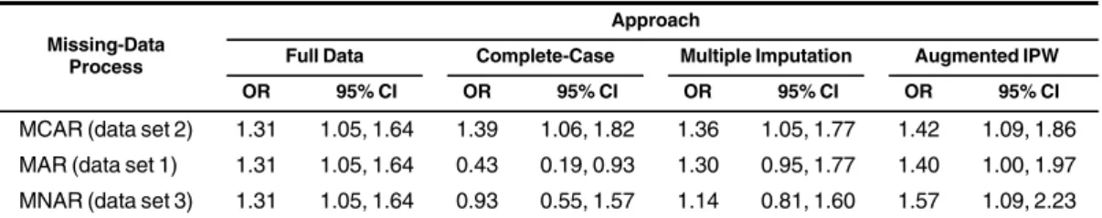
In the corresponding companion papers (14,15), the analyti-cal teams closely mimicked the real-world application of these missing-data methods because the underlying mechanism used to create the missing data is rarely known in practice and was not known to the investigators in this exercise. The results from the analyses are unmasked here and consolidated in Table4, along with the (“true”) results from the full data. The“Full Data”column represents the association of smoking with spon-taneous abortion after adjustment for race, age, and BMI in the complete subsample from the CPP cohort, showing an odds ratio of 1.31 (95% confidence interval: 1.05, 1.64) for all 3 data sets. The rows of Table4correspond to the data sets in which a given missing-data mechanism was imposed. Results are pro-vided for complete-case analyses, MI, and augmented IPW, along with the results from the full data. Of course, some varia-tion in the point estimates will be expected even for unbiased sce-narios due to sampling variability, as these are single realizations of the data.
For MCAR (i.e., data set 2 in the companion papers), complete-case analyses and use of both principled methods re-sulted in similar point estimates and confidence intervals. For this realization of the data, all 3 methods estimated odds ratios that were close to those from the full data, with slightly wider confi -dence intervals, reflecting the loss of information due to the miss-ing data, essentially a consequence of a reduced sample size.
For the MAR mechanism (i.e., data set 1 in the companion pa-pers), the complete-case analysis estimate of 0.43 shows a nota-ble and spurious protective effect of smoking on spontaneous abortion. This effect reversal is primarily due to the violated assumption that the missingness is MCAR, when in fact it is a function of the observed variables. In some settings, complete-case analysis can be valid under MAR and even MNAR—for example, if the missingness process depends only on covar-iates in the regression, even if some of them are not fully observed (26). However, this assumption is not met in our exam-ple, which serves to highlight the potential consequences of applying complete-case analysis and subsequently failing to address the impact of the missing data. On the other hand, em-ploying either MI or augmented IPW resulted in point esti-mates of 1.30 and 1.40, respectively, with similar confidence intervals. Both estimates showed a drastic shift from the (naive)
Table 4. Estimated Odds Ratiosafor the Association Between Smoking and Spontaneous Abortion According to
Data Analysis Approach, Collaborative Perinatal Project, 1959–1965
Missing-Data Process
Approach
Full Data Complete-Case Multiple Imputation Augmented IPW
OR 95% CI OR 95% CI OR 95% CI OR 95% CI
MCAR (data set 2) 1.31 1.05, 1.64 1.39 1.06, 1.82 1.36 1.05, 1.77 1.42 1.09, 1.86
MAR (data set 1) 1.31 1.05, 1.64 0.43 0.19, 0.93 1.30 0.95, 1.77 1.40 1.00, 1.97
MNAR (data set 3) 1.31 1.05, 1.64 0.93 0.55, 1.57 1.14 0.81, 1.60 1.57 1.09, 2.23
Abbreviations: CI, confidence interval; IPW, inverse probability weighting; MAR, missing at random; MCAR,
miss-ing completely at random; MNAR, missmiss-ing not at random; OR, odds ratio.
Rather, all available and relevant data should be used to impute or model the missingness mechanism, regardless of its temporal relationship to the exposure or outcome. For instance, there may be observed variables that are highly predictive of the missing variables or the missingness mechanism but do not enter into the analysis model, either because they are not predictive of the out-come or because they are not confounders. These auxiliary vari-ables are beneficial and easy to use in MI and are considered one of the advantages of the method. In this exercise, only variables chosen a priori to be included in the analysis model were avail-able, implying that the variable sets for the imputation and analy-sis models were the same.
In contrast to MI, IPW assumes that a model for the nonre-sponse process given the observed data is correctly specified. Because the model for the missing-data process does not restrict the model of substantive interest and vice versa, IPW (and augmented IPW) is not limited by a compatibility of con-ditional densities under the MAR assumption. However, IPW requires that for all possible realizations of the full data, there is a nonzero probability of observing a person with complete data (i.e., the positivity assumption) (29). IPW as implemen-ted here relies on large-sample theory for valid inference. In practice, MI-based inference also often relies on large-sample inference (30–32). However, when proper imputation is applied under a strict Bayesian framework (implying no Pvalues or confidence intervals), MI can in principle be applied in small samples as well, so long as additional assumptions concern-ing the fully conditional distribution hold.
In actuality, MI and IPW make somewhat complementary modeling assumptions, as they rely on parametric models for distinct components of the joint likelihood for the full data and the missingness process. As stated above, MI relies on a model for the underlying full data but allows the missingness mechanism to remain completely unrestricted. Conversely, IPW models the missingness mechanism, but the full-data model is unrestricted beyond the model of substantive interest. As with a complete-case analysis, IPW does not efficiently use information available in incomplete cases, although these data are used to estimate the nonresponse rates, therefore recovering some information from incomplete cases. This issue does not arise with MI because available information among incom-plete cases serves as a basis for imputing missing information. In the other companion paper, Sun et al. (15) considered an augmented IPW, an extension of IPW attributable to Robins et al. (29) and recently implemented for nonmonotone MAR patterns by Sun and Tchetgen Tchetgen (33), which largely resolves the efficiency limitation of standard IPW by allow-ing the analyst to recover information in incomplete cases.
DISCUSSION
Based on the above considerations, complete-case analysis should be used with the same caution we ascribe to unadjusted estimates, as its validity relies on strong, often unrealistic as-sumptions. In contrast, principled methods such as MI or IPW may account for bias due to missing data under weaker assump-tions. The most standard application of these methods relies on the MAR assumption. In the absence of model misspecification, we expect that MI will be more efficient than IPW, because the complete-caseanalysesestimatetowardtheeffectobservedin
thefulldata.
FortheMNARcase(i.e.,dataset3inthecompanion pa-pers), complete-case analyses resulted in an estimated odds ratioof0.93(95%confidenceinterval:0.55,1.57).Whileboth MIandIPWresultedinpointestimatesclosertothefull-data effectestimate,suchafindingcannotbeexpectedgenerally.
PRINCIPLEDMETHODS:PROS,CONS,AND ASSUMPTIONS
Ingeneral, standardcomplete-case analysesrelyonan assumptionthatthemissingdataareMCARoranequivalent assumptiontoyieldunbiasedestimates(26).Thisassumption mayoftenbeunrealisticinepidemiologicsettings,inwhich complete-caseanalyseswilllikelyresultinbias(e.g.,dataset2). Furthermore,evenifdataareMCAR,suchacomplete-case analysiswilltypicallybeinefficient,asitignoresvaluable infor-mationinincompletecases,whichcanbeparticularly dele-terious when a necessary covariate is the predominantly missingvariable.
WhendataareMAR,bothMIandIPWmaystillreturn unbi-asedestimateswhenappropriateassumptionsaremet.In partic-ular,standardMIandIPWasimplementedinthecompanion papers(14,15)relyonspecificmodelingassumptionsbeyond assuming anignorablenonresponse process(27). MIis for-mallyaBayesianapproachwhich,asimplementedinthe com-panionpaperbyHareletal.(14),assumesthattheparameters indexingmodelsofinteresthave anormalpriordistribution. Theimputationmodelandtheanalysismodelarealsoassumed tobecorrectlyspecified,whichincludescorrectspecificationof theconditionaldistributionofincompletevariablesgiventhe observedvariables.Thisalsoimpliesthattheimputationmodel forthedistributionofcovariatesgiventheoutcomeis compati-blewiththeunderlyingmodelofsubstantiveinterest forthe densityoftheoutcomegivencovariates.Thisisguaranteedto occurwhenthejointdistributionofthecovariatesandoutcome isjointnormalandforcertainmodelchoiceswithinthenatural exponentialfamily,butnotingeneral.
Therearedifferenttypesofimputationmodels;somerequire parametricassumptions(e.g.,jointnormaldistributioninMI) andsomedonot(e.g.,hot-deck).Whilemisspecifiedmodels shouldnotbeexpectedtoproduceunbiasedresults,simulations haveshownthatMIissomewhatrobusttothechoiceof imputa-tionmodelformoderateratesofmissinginformation.AllMI im-plementedbyHareletal.inthecompanionpaper(14) used a “proper”parametricimputationmodel,whichrespectsthe distri-butionalpropertiesoftheimputationdraws,typicallyby draw-ingvaluesofparametersbeforedrawingimputations(12,28).
latter assumes that the full-data model is completely unre-stricted other than by the model of substantive interest, while the former uses a restricted parametric formulation for the full data (29,30). While IPW fails to efficiently recover all available information from incomplete cases, augmented IPW recovers such information, at least the portion recoverable without rely-ing on afinite-dimension full-data model.
Now, given that we wish to use principled methods, which are we to choose? We can choose a version of MI, a version of IPW, or another formal approach not considered in this set of articles (e.g., direct maximum likelihood, Bayesian analysis) that equally applies under MAR. We believe foremost that we should prioritize a consistent estimator under ignorable MAR settings. Then, to the extent possible, we should minimize var-iance, although reasonable tradeoffs in allowing some bias in exchange for increased precision may be prudent (e.g., to min-imize mean squared error). We remain without consensus as to the extent to whichflexible parametric models may be overly restrictive and hide some amount of estimation error, but we do have consensus that low-dimension parametric models can be overly restrictive and hinder our ability to see the world more clearly: In such cases, in our results we might see more of our assumptions than we see of our world (1). Indeed, nuisance models required for controlling selection bias (e.g., the imputation model, the missing-data mechanism model) do not need to return interpretable finite-dimension parameters, and therefore they might be restricted only by the requirement to achieve a consistent estimator of the parameter(s) of interest from the substantive model.
This leaves us the ability to pick from several candidate methods. Some of these candidate methods have nonoverlap-ping assumptions, as mentioned above. Therefore, there should be advantages to conducting more than 1 analysis and compar-ing results, as we have done with IPW and MI. When results with nonoverlapping assumptions agree, then our confidence in the results should be higher—emboldened, but never cer-tain, because even nonoverlapping assumptions may jointly fail. When results disagree, we should pause and reconsider our assumptions and methods.
Current research on missing data is producing moreflexible procedures, such as doubly robust estimators, that combine a model for the full data with a model for the missing-data pro-cess, such that only 1 of the models need be correctly specified to produce unbiased inferences. While the advent of accessible software packages for these methods may be on the horizon, moving away from complete-case analysis towards a principled method like MI or IPW as demonstrated in the companion pa-pers (14,15) is vital to ensuring proper analysis of current epi-demiologic studies.
When analyzing observational data, an epidemiologist presented with a crude odds ratio of 0.43 (analogous to the complete-case analysis estimate) and an adjusted odds ratio of 1.35 (analogous to MI or IPW estimate) might posit that con-founding bias is the culprit and report both, while interpreting the adjusted result as probably closer to the underlying truth (barring collider-stratification bias and assuming a rare out-come such that the odds ratio is collapsible). Reporting only the results from a complete-case analysis in the presence of nontrivial missing data is commensurate with reporting only crude associations from nonrandomized studies. We therefore
advocate that the same reasoning be followed when dealing with missing data. If we are principled, we are more likely to get closer to the truth.
We urge researchers, reviewers, and journal editors to think about the missing-data problem prior to making decisions about a plan of action. We would be wise to plan for missing values, minimize nonresponse, determine the missing-data as-sumptions, and report them appropriately. Of course, there may be reasonable extenuating circumstances that support reporting a crude association, or an equivalent rationale for reporting re-sults from a complete-case analysis. But we surmise that such cases are rare. In closing, we ask that researchers join us in re-evaluating the context of our work, to think more carefully about the assumptions that underlie the claims we make.
ACKNOWLEDGMENTS
Author affiliations: Division of Intramural Population Health Research, Eunice Kennedy Shriver National Institute of Child Health and Human Development, Rockville, Maryland (Neil J. Perkins, Enrique F. Schisterman); Department of Epidemiology, Gillings School of Global Public Health, University of North Carolina at Chapel Hill, Chapel Hill, North Carolina (Stephen R. Cole); Department of Statistics, College of Liberal Arts and Sciences,
University of Connecticut, Storrs, Connecticut (Ofer Harel); Department of Biostatistics, Harvard T.H. Chan School of Public Health, Boston, Massachusetts (Eric J. Tchetgen Tchetgen, BaoLuo Sun); and Agency for Healthcare Research and Quality, Rockville, Maryland (Emily M. Mitchell).
This research was partially supported by the Long-Range Research Initiative of the American Chemistry Council (Washington, DC) and the Intramural Research Program of theEunice Kennedy ShriverNational Institute of Child Health and Human Development, National Institutes of Health. This work was also partially supported by award K01MH087219 from the National Institute of Mental Health.
The content of this article is solely the responsibility of the authors and does not necessarily represent the official views of the National Institute of Mental Health or the National Institutes of Health.
Conflict of interest: none declared.
REFERENCES
1. Little RJ, D’Agostino R, Cohen ML, et al. The prevention and treatment of missing data in clinical trials.N Engl J Med. 2012; 367(14):1355–1360.
2. Eekhout I, de Boer RM, Twisk JW, et al. Missing data: a systematic review of how they are reported and handled. Epidemiology. 2012;23(5):729–732.
3. Harel O, Boyko J. Mi??ing data: should we c?re?Am J Public Health. 2013;103(2):200–201.
5. Sterne JA, White IR, Carlin JB, et al. Multiple imputation for missing data in epidemiological and clinical research: potential and pitfalls.BMJ. 2009;338:b2393.
6. Stuart EA, Azur M, Frangakis C, et al. Multiple imputation with large data sets: a case study of the Children’s Mental Health Initiative.Am J Epidemiol. 2009;169(9):1133–1139. 7. van der Heijden GJ, Donders AR, Stijnen T, et al. Imputation of
missing values is superior to complete case analysis and the missing-indicator method in multivariable diagnostic research: a clinical example.J Clin Epidemiol. 2006;59(10):1102–1109. 8. Westreich D. Berkson’s bias, selection bias, and missing data.
Epidemiology. 2012;23(1):159–164.
9. Wood AM, White IR, Thompson SG. Are missing outcome data adequately handled? A review of published randomized controlled trials in major medical journals.Clin Trials. 2004; 1(4):368–376.
10. Harel O, Pellowski J, Kalichman S. Are we missing the importance of missing values in HIV prevention randomized clinical trials? Review and recommendations.AIDS Behav. 2012;16(6):1382–1393.
11. Allison PD.Missing Data. Thousand Oaks, CA: SAGE Publishing; 2002.
12. Schafer JL.Analysis of Incomplete Multivariate Data. New York, NY: Chapman & Hall, Inc.; 1997.
13. Hardy JB. The Collaborative Perinatal Project: lessons and legacy.Ann Epidemiol. 2003;13(5):303–311.
14. Harel O, Mitchell EM, Perkins NJ, et al. Multiple imputation for incomplete data in epidemiologic studies.Am J Epidemiol. 2018;187(3):576–584.
15. Sun BL, Perkins NJ, Cole SR, et al. Inverse-probability-weighted estimation for monotone and nonmonotone missing data.Am J Epidemiol. 2018;187(3):585–591.
16. Rubin DB. Inference and missing data.Biometrika. 1976; 63(3):581–590.
17. Rubin DB.Multiple Imputation for Nonresponse in Surveys. New York, NY: John Wiley & Sons, Inc.; 1987.
18. Gill RD, van der Lann MJ, Robins JM. Coarsening at random: characterizations, conjectures, counter-examples. In: Lin DY, Fleming TR, eds.Proceedings of the First Seattle Symposium in Biostatistics: Survival Analysis. (Lecture Notes in Statistics, vol. 123). New York, NY: Springer-Verlag New York; 1997: 255–294.
19. Molenberghs G, Kenward MG.Missing Data in Clinical Studies. 1st ed. New York, NY: John Wiley & Sons, Inc.; 2007. 20. Siddique J, Harel O, Crespi CM. Addressing missing data
mechanism uncertainty using multiple-model multiple imputation: application to a longitudinal clinical trial.Ann Appl Stat. 2012;6(4):1814–1837.
21. Daniels MJ, Hogan JW.Missing Data in Longitudinal Studies: Strategies for Bayesian Modeling and Sensitivity Analysis. Boca Raton, FL: Chapman & Hall/CRC Press; 2008. 22. Daniel RM, Kenward MG, Cousens SN, et al. Using causal
diagrams to guide analysis in missing data problems.Stat Methods Med Res. 2012;21(3):243–256.
23. Pearl J.Causality: Models, Reasoning, and Interence. New York, NY: Cambridge University Press; 2000.
24. Little RJ, Zanganeh SZ. Missing at random and ignorability for inferences about subsets of parameters with missing data. (University of Michigan Department of Biostatistics Working Paper Series, working paper 98). Ann Arbor, MI: University of Michigan; 2013.http://biostats.bepress.com/umichbiostat/ paper98/. Accessed December 15, 2015.
25. Little RJ. Pattern-mixture models for multivariate incomplete data.J Am Stat Assoc. 1993;88(421):125–134.
26. Bartlett JW, Harel O, Carpenter JR. Asymptotically unbiased estimation of exposure odds ratios in complete records logistic regression.Am J Epidemiol. 2015;182(8):730–736.
27. Little RJ, Rubin DB.Statistical Analysis With Missing Data. New York, NY: John Wiley & Sons, Inc.; 1987.
28. Rubin DB. Multiple imputation after 18+years.J Am Stat Assoc. 1996;91(434):473–489.
29. Robins JM, Rotnitzky A, Zhao LP. Estimation of regression coefficients when some regressors are not always observed. J Am Stat Assoc. 1994;89(427):846–866.
30. Tsiatis AA.Semiparametric Theory and Missing Data. 1st ed. New York, NY: Springer-Verlag New York; 2006.
31. Robins JM, Wang N. Inference for imputation estimators. Biometrika. 2000;87(1):113–124.
32. Wang N, Robins JM. Large-sample theory for parametric multiple imputation procedures.Biometrika. 1998;85(4): 935–948.
33. Sun BL, Tchetgen Tchetgen EJ. On inverse probability weighting for nonmonotone missing at random data.arXiv.org.