Sharif University of Technology
Scientia IranicaTransactions A: Civil Engineering www.scientiairanica.com
Research Note
Structural optimization by spherical interpolation of
objective function and constraints
H. Meshki
aand A. Joghataie
b;a. Department of Civil Engineering, Science and Research Branch, Islamic Azad University, Tehran, P.O. Box 14515-775, Iran. b. Department of Civil Engineering, Sharif University of Technology, Tehran, P.O. Box 11155-9313, Iran.
Received 10 June 2014; received in revised form 14 March 2015; accepted 13 September 2015
KEYWORDS Spherical interpolation; n-dimensional sphere; Radius of curvature; Reference point; Lagrange multipliers; Constrained problems.
Abstract. A new method for structural optimization is presented for successive approximation of the objective function and constraints in conjunction with Lagrange multipliers approach. The focus is on presenting the methodology with simple examples. The basis of the iterative algorithm is that after each iteration, it brings the approximate location of the estimated minimum closer to the exact location, gradually. In other words, instead of the linear or parabolic term used in Taylor expansion, which works based on a short step length, an arch is used that has a constant curvature but a longer step length. Using this approximation, the equations of optimization involve the Lagrange multipliers as the only unknown variables. The equations which depend on the design variables are decoupled linearly as these variables are directly obtained. One mathematical example is solved to explain in details how the method works. Next, the method is applied to the optimization of a simple truss structure to explain how the method can be used in structural optimization. The same problems have been solved by penalty method and compared. The results from both methods have been the same. However, because of the long step length and reduction in the number of variables, the speed of convergence has been higher in the presented method.
© 2016 Sharif University of Technology. All rights reserved.
1. Introduction
In a real structural engineering problem with a large number of variables, the cost of numerical iterations for optimization is generally high. In this paper, Lagrange method, which is a subset of the direct optimization methods, has been used. A problem with direct optimization techniques is the number of constraints, which can be large for applied problems. For example, in Sequential Linear Programming [1], which is a widely used direct optimization method [2-5], the problem is formulated to be solved using simplex
*. Corresponding author. Tel.: +98 21 66164216 E-mail addresses: [email protected] (H. Meshki); [email protected] (A. Joghataie)
algorithm. This requires working with not only the main constraints, but also additional constraints on the upper and lower limits of the variables, which can increase the total number of constraints, signicantly, for problems with a large number of variables [6], or in sequential quadratic programming [7-9], the number of constraints is at least equal to the sum of the number of design variables and the Lagrange multi-pliers, which can make the procedure of optimization very time-taking. However, in the method presented in this paper, because the constraints and objective function are replaced with their equivalent spheres, the problem is discretized into several independent sub-problems which are solved independently to provide an approximate solution. Through successive iterations, the solution is obtained. This characteristic of the
method results in the increase in the speed of conver-gence.
In methods such as the sequential linear pro-gramming [2,10] and the sequential quadratic program-ming [6,11-13], Taylor expansion is used for interpola-tion of the funcinterpola-tions, while in the method presented here, the functions are approximated by spheres in the n-dimensional space for n-dimensional problems. Hence, the method uses the radii of curvature, which are the radii of the spheres which are tangent to the given n-dimensional functions of constraints and objective function. At the tangent point of each of the spheres to its corresponding function, the curvature is determined based on the gradient of the function at the tangent point. Obviously, the gradient passes through the center of the sphere. This simple approximation makes the convergence become faster. After the spheres are determined, through a simple optimization algorithm, an optimum point for the system of spheres is determined. Next, the optimum point is projected back on the original functions and the procedure is repeated until convergence is achieved.
In the next sections, to provide an easy and better explanation of the method, rst, the method and for-mulation are explained and discussed for 2-dimensional problems, based on which the general formulation and method is presented. Several examples are included to show how the method can be used to solve analytical and numerical problems. The results of numerical problems are compared with the results obtained from exterior penalty method. Since this is the rst paper on the method, the main goal has been to present the formulation and its capability in solving a number of test problems. There are steps which should be taken to assess the dierent features of this method, including its convergence behaviour, and to determine the group of problems where application of this method is advantageous, though a better convergence speed has already been observed in the demonstration examples solved in this paper, as compared with the exterior penalty method.
2. Two-dimensional problems
Though the general mathematical model will be pre-sented in the next section, in this section, for better clarication and simpler explanation of the spherical approximation method, the basic procedure for 2-dimentional optimization problems is presented graph-ically as shown in Figure 1.
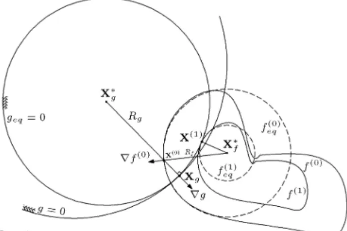
In Figure 1, X(0) is the initial point, which is
used to nd the point Xg on the active constraint
g = 0, which is also at the nearest distance from point X(0). To obtain point X
g, a normal is drawn from
X(0) to the constraint g = 0, where the tangent point
is denoted by Xg. Clearly, the vector connecting point
Figure 1. Procedure of updating reference point X(0) to X(1).
X(0) to Xg aligns with the gradient of g = 0 at point
Xg, denoted by V g. The radius of curvature of the
constraint at Xg is denoted by Rg. Now, using X(0),
Xg, and Rg, it is possible to determine the center of the
circle (sphere) denoted by Xg, as shown in Figure 1.
The original constraint g = 0 is now approximated with an equivalent constraint geq= 0, which is circular
(spherical). Similarly, using the same point of X(0), it
is possible to construct for the objective function, f(x), an equivalent circular (spherical) objective function, which is denoted by feq(0).
However, the circle is constructed so that X(0) is
the tangent point, as shown in Figure 1. Denoting the radius of curvature of the objective function by Rf and
its gradient by V f at point X(0), the center of sphere
of the objective function, X
f, can be obtained. Having
the equivalent constraint, geq = 0, and the sphere
center of the objective function, X
f can be obtained,
which is the intersection point of the line connecting the two centers of the equivalent constraint and objective function. X(1) is now considered to be the starting
point for the next iteration. It is noteworthy that X(1)
is the tangent point of the two circles (spheres).
3. General multivariable problems
The general form of the optimization problems studied in this paper is:
min f = f(X); (1) s.t.
gi(X) 0 j = 1; 2; :::; m; (2)
gj(X) = 0 j = m + 1; 2; :::; p; (3)
where m denotes the number of inequality constraints and p is the number of equality constraints.
An n-dimensional spherical interpolation problem can be expressed as follows:
min f =
n
X
i=1
xi xif
2 R2
f+ f(X(k)); (4)
s.t.
gj(X) = n
X
i=1
xi xij
2 R2
j 0 j = 1; 2; :::; m;
(5)
gj(X) = n
X
i=1
xi xij
2 R2
j = 0 j = m + 1; :::; p;
(6) where k is iteration number; n, number of variables; xi, the ith design variable; xif, the ith component of
the center point of the objective function equivalent sphere, x
ij, the ith component of the center point
of the jth constraint equivalent sphere; Rf, radius
of the objective function sphere; Rj, radius of the
jth constraint sphere; and f(X(k)), objective function
value in the kth iteration.
3.1. Determining the approximate parameters 3.1.1. Radius of the spheres in the n-dimensional
space
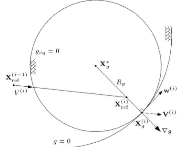
The radius of curvature can be determined based on the denition of curvature as the ratio of arch length to the angle of curvature. Since the angle of curvature occurs in a specic plane, rst, a plane specied with two vectors in the n-dimensional space should be dened. In other words, for every point on an n-dimensional function surface, a curvature exists for every specic direction. Since the radius of curvature is perpendic-ular to the surface, it points toward the gradient of the surface, which is in the same direction as that of the radius of curvature. Also, since the reference point moves toward the optimal point in sequential steps, the radius of curvature should be calculated along the vector connecting the two subsequent reference points according to Figure 2, where V(i) shows the vector.
Therefore, the plane of curvature includes both V(i)
and the gradient vector, V g. Since basically path of arch length is tangent to surface, it is assumed that the vector w(i), which is tangent to the surface (or
perpendicular to V g) and is in the plane of V(i) and
V g, is replaced instead of vector V(i), based on which
the radius of curvature is determined in the direction of w(i). As it will be illustrated, use of w(i) instead
of V(i) causes simplication of the calculations. First,
vector w(i) is obtained as described below:
In the ith computational step, according to Fig-ure 2, V(i)is dened as the optimal path vector, which
is obtained by connecting the two subsequent reference points Xref(i) and Xref(i 1) as:
V(i)= x(i)ref x(i 1)ref
kx(i)ref x(i 1)ref k: (7)
Figure 2. Constraint's radius of curvature, Rg, toward w(i); vector w(i)in plane of two vectors V(i)and V g, and also V(i)in direction of two sequent reference points, X(i) ref rand X(i 1)
ref .
Basically, the n 1 vectors, denoted by w1; w2; :::;
wn 1, which have the property to be orthogonal to V
in the n-dimensional space, [14] are as follows:
wn 1=V hwhV; w1i 1; w1iw1 :::
hV; wn 2i
hwn 2; wn 2iwn 2(8);
where, sign hi is the inner product operator.
However, for the specic vectors V and V g, the tangential vector w0, which is perpendicular to V g and
is also in the plane of the two vectors V and V g, is:
w0= V hrg; rgihV; rgirg (9)
w0 is normalized to provide a unit vector in the same
direction as follows: w = w0
kw0k: (10)
Based on the previous denition of curvature, the radius of curvature is equal to the ratio of the change in arch length to the change in curvature angle in the direction of w. The unit gradient vector bG normal to the surface is dened as:
b
G = krgkrg : (11)
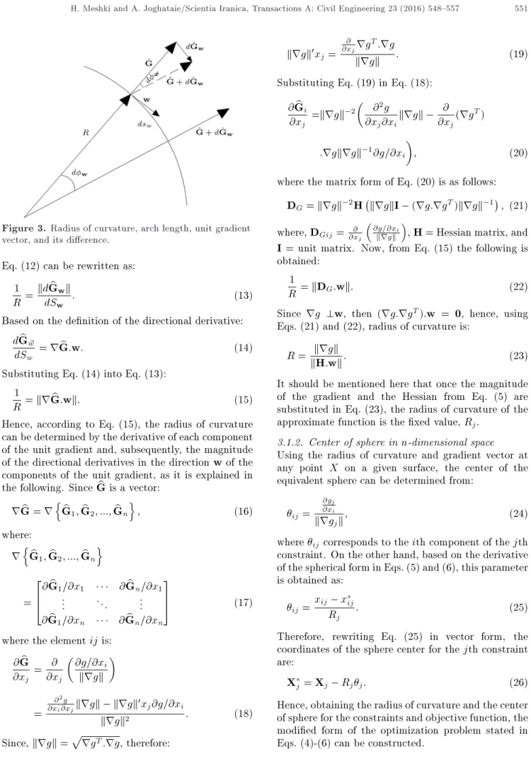
Then, by applying a simple proportioning according to Figure 3:
dw~ = dSRw = kd bGwk
k bGk ; (12) where, w is curvature angle toward the direction w,
and Sw is arch length in the direction of w.
Figure 3. Radius of curvature, arch length, unit gradient vector, and its dierence.
Eq. (12) can be rewritten as: 1
R =
kd bGwk
dSw : (13)
Based on the denition of the directional derivative: d bGw~
dSw = r bG:w: (14)
Substituting Eq. (14) into Eq. (13): 1
R = kr bG:wk: (15) Hence, according to Eq. (15), the radius of curvature can be determined by the derivative of each component of the unit gradient and, subsequently, the magnitude of the directional derivatives in the direction w of the components of the unit gradient, as it is explained in the following. Since bG is a vector:
r bG = rnGb1; bG2; :::; bGn
o
; (16)
where:
rnGb1; bG2; :::; bGn
o
= 2 6 4
@ bG1=@x1 @ bGn=@x1
... ... ... @ bG1=@xn @ bGn=@xn
3 7
5 (17)
where the element ij is: @ bG
@xj =
@ @xj
@g=@xi
krgk
=
@2g
@xi@xjkrgk krgk
0xj@g=@xi
krgk2 : (18)
Since, krgk =prgT:rg, therefore:
krgk0x j=
@ @xjrg
T:rg
krgk : (19)
Substituting Eq. (19) in Eq. (18): @ bGi
@xj =krgk
2 @2g
@xj@xikrgk
@ @xj(rg
T)
:rgkrgk 1@g=@x i
; (20)
where the matrix form of Eq. (20) is as follows: DG= krgk 2H krgkI (rg:rgT)krgk 1; (21)
where, DGij =@x@j
@g=@xi
krgk
, H = Hessian matrix, and I = unit matrix. Now, from Eq. (15) the following is obtained:
1
R = kDG:wk: (22) Since rg ?w, then (rg:rgT):w = 0, hence, using
Eqs. (21) and (22), radius of curvature is:
R = kH:wkkrgk : (23)
It should be mentioned here that once the magnitude of the gradient and the Hessian from Eq. (5) are substituted in Eq. (23), the radius of curvature of the approximate function is the xed value, Rj.
3.1.2. Center of sphere in n-dimensional space Using the radius of curvature and gradient vector at any point X on a given surface, the center of the equivalent sphere can be determined from:
ij = @gj
@xi
krgjk; (24)
where ij corresponds to the ith component of the jth
constraint. On the other hand, based on the derivative of the spherical form in Eqs. (5) and (6), this parameter is obtained as:
ij =xij x ij
Rj : (25)
Therefore, rewriting Eq. (25) in vector form, the coordinates of the sphere center for the jth constraint are:
X
j = Xj Rjj: (26)
Hence, obtaining the radius of curvature and the center of sphere for the constraints and objective function, the modied form of the optimization problem stated in Eqs. (4)-(6) can be constructed.
3.2. Updating the reference point
Following Eqs. (4)-(6), the Lagrange function can be written as follows:
minxL = f + m
X
j=1
jgj; (27)
where f is the objective function; gj, the jth constraint;
and j, Lagrange multiplier.
For the inequality constraints gj 0, the solution
technique is the active constraint method. At the rst step, all the constraints are assumed active where all of them are considered to be the equality constraints. For the solution to be a minimum according to Kuhn-Tucker conditions, the multiplier(s) should be positive. Obtaining the Lagrange multiplier, if the constraint multiplier is negative, the constraint related to the most negative multiplier is eliminated and the cal-culation is repeated until according to Kuhn-Tucker conditions, there remains non-positive multiplier.
Using Lagrange equation @L
@xi = 0 for Eq. (27), the
following is obtained: @f
@xi + m
X
j=1
j@g@xj
i = 0: (28)
Here, substituting the approximate spheres for f and gj as discussed in Eqs. (4)-(6) and also Eq. (25):
@L
@xi = 2 xi x if
+ 2Xm
j=1
j xi xij
= 0: (29)
The variable xi is obtained from Eq. (29) as:
xi= x if +
Pm
j=1(jxij)
1 +Pmj=1(j) : (30)
Since the denominator of Eq. (30) is a scalar quantity, the vector of design variable X is obtained as follows:
X = X
f+ Xnm
= 1 + 1T; (31)
where the components of matrix X and vector X f,
respectively, are x
ij and xif. In the next section, the
multiplier vector in Eq. (31) is obtained. 3.3. Determining Lagrange multipliers for
constraints
Using the last Lagrange equation @L @j = 0:
n
X
i=1
xi xij
2= R2
j; j = 1; 2; :::; m; (32)
where, m is the number of active constraints: The vector form of Eq. (32) is:
X X j
T X X j
= R2
j: (33)
Rewriting Eq. (33) gives:
XTX 2XTX
j+ XTj Xj = R2j: (34)
Substituting Eq. (31) in Eq. (34) gives: XT
f Xf+ 2XTf X + XTX
2 XT
f Xj+ XTj X
1 + 1T m1
+ XT
j Xj R2j
1 + 1T m1
2
= 0: (35) The last parenthesis in Eq. (35) can be written as:
1 + 1T m1
2
= 1 + T1
mm + 21Tm1: (36)
Therefore, rewriting Eq. (35) and using Eq. (36) the following is obtained:
gj= TAj + BTj + Cj = 0; j = 1; 2; :::; m;
(37) where:
Aj=XTX 2 Xj1Tm1
TX
+ XT
j Xj R2j
1mm; (38)
BT
j = 2 Xf Xj
T X X j1Tm1
2R2
j1Tm1;
(39) Cj = Xf Xj
TX f Xj
R2
j: (40)
Using the m Eqs. in (37),
g = A+ BT + C = 0; (41)
where:
A;j= TAj: (42)
The Lagrange multipliers can be obtained by one of the numerical methods such as the Jacobean technique for the matrix equation (41).
3.4. Returning the reference point to constraint surface
Using the previous relations, the radius of curvature and center of sphere for the objective function and the constraints can be determined. For the objective func-tion, these calculations are performed at the reference point, but for the constraints, because they are xed in the n-dimensional space and on the other hand the constraints themselves are not approximated but their curvatures are approximated, rst, the reference point is returned to all the active constraints; then, at these points, the approximate parameters are calculated. The criterion for returning to the active constraint is based on the shortest distance of the reference point from each of the active constraints, because the
reference point is the basis for optimization calcula-tions obtained by Lagrange equacalcula-tions. Hence, every computational step includes two parts: determination of the reference point and its returning to the surface of active constraints. The shortest distance between the reference point and each of the active constraints is obtained based on the following optimization problem:
minxlj(X)2=
Xj X(k)ref
T
Xj X(k)ref
: (43) s.t.
gj(x) = 0; (44)
where, lj(X) is direction vector between Xj and X(k)ref;
X(k)ref, coordinate of reference point in the kth iteration; and Xj, point coordinate on the jth active constraint
and with the shortest distance from the reference point. To solve the above problem, the following method is performed. Substituting the Lagrange function as:
= l2
j+ gj; (45)
in the Lagrange equation, r = 0 can be written as: 2lj = rgj: (46)
Multiplying the left and right sides of Eq. (46) by their own transposes,
4l2
j = 2rgjTrgj; and = 4lj2=rgjTrgj60:5; (47)
is plugged in Eq. (46) to obtain the vector Xj in
iteration i + 1: X(i+1)j = krgkljk
jkrgj
X(i)j
+X(k)ref: (48)
In Eqs. (44) and (48), For k = 1, where the reference point is Xref(0), the initial point Xj(0) is selected as:
X(0)j = X(0)ref+ X; (49) where X is arbitrary vector with small values.
For the next iterations, when k > 1, the point obtained on the jth constraint at iteration k 1 can be chosen as the initial point X(0)j . Now, according to Eq. (43), the direction vector l(1)j (X), which according to Eq. (46) or (48) has the same line of action of gj,
is determined from l(1)j (X) = X(0)j X(k)ref. Also X(1)j is on the same line; so, X(1)j = l(1)j (X) + X(0)j , which is inserted in Eq. (51) for gj (X(1)j ) = 0 to obtain and,
consequently, X(1)j . At the next step, X(1)j is used in Eq. (55) to determine if X(2)j is obtained.
This procedure is repeated until the exact solution is obtained, so that X(i+1)j in iteration i+1 is placed on the jth active constraint and at the shortest distance from the reference point X(k)ref.
4. Spherical optimization algorithm
Based on the equations explained in the previous sections, an algorithm is developed, which is explained in this section. Also, two examples are solved by this algorithm, which is reported in the next section. Briey, the algorithm is:
(a) Select an initial feasible reference point, denoted by X(0);
(b) For each of the constraints, return the reference point to the surface of the constraint, following Eqs. (44) and (48) and according to Sections 3 and 4;
(c) Obtain the approximate objective function at the reference point and also the approximate con-straints at the points obtained at step (b) using Eqs. (23) and (26) according to Section 3.1 of this paper, explained before;
(d) Construct and solve the system of Lagrange mul-tiplier equations according to Eqs. (38)-(41) and Section 3.3 and also using the parameters of the spherical functions obtained at step (c);
(e) Eliminate the most negative Lagrange multiplier and its constraint from the system of Lagrange multiplier equations from step (d) by eliminating the rows and columns corresponding to coecients A, B, and C related to the most negative Lagrange multipliers represented in Eqs. (38)-(40). Repeat the previous steps until all the remaining Lagrange multipliers are non-negative;
(f) Determine the reference point using Eq. (31);
(g) If either the reference point is at the intersection of all the active original constraints or convergence has been achieved according to the following cri-teria for monitoring the change in the location of two successive reference points as:
e = kX(i)ref X(i 1)ref k 2; (50) then terminate; where, 2 is small value, X(i)ref is reference point at the ith step;
(h) Otherwise select the latter reference point as the new initial point and go to step (b) and repeat the previous steps.
5. Example problems
Two examples, which cover simple to complicated cases, are solved by the algorithm and the results are compared with widely used optimization methods, in-cluding the penalty method and the active-set method, according to Matlab software.
5.1. Example-1: Objective function with 3 variables subject to 2 constraints
This example has 3 variables subject to 2 constraints. The problem is:
minxF = 2x1+ 5x22 7x23; (51)
s.t.
g1= x3 5xx1
2 1 0; (52)
g2= 2x21 3x2+ x33 10 0: (53)
First, using a commercial optimization software and employing another optimization method and starting from the initial point X(0)= (2; 2; 2), the problem was
solved and the optimal point was obtained as Xopt =
(0:1348; 0:5343; 2:2615), where Fopt = 34:1045.
Sub-sequently, solving the problem by the spherical op-timization method, the result of the problem was obtained as in Table 1.
Using Eqs. (44) and (48), the points on the 2 constraints, with the shortest distance from reference point have been obtained. Next, using Eqs. (9) and (10), the tangential vector, w, related to the 2 successive reference points for the objective function and the 2 constraints have been obtained. Then, using Eqs. (23) and (26), the radius of curvature and center of sphere for the objective function and the 2 constraints have been calculated.
As can be seen in Table 1, the distances of both constraints from the reference point have decreased step by step, monotonically. Both of the Lagrange multipliers are positive at all the steps. This shows that both constraints have been active in all the solution steps. The fast variation of error values in Table 1 illustrates a good convergence in this method.
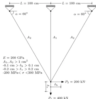
Figure 4. Truss optimization problem where the cross-sectional areas should be determined for minimum weight, subject to minimum area of sections,
displacement, and stress constraints.
5.2. Example 2: Structural example
This is a numerical structural optimization problem. The structure is the steel truss shown in Figure 4, where the elasticity modulus is E = 200 GPa.
The problem is formulated as:
minA1;A2f = hA1+ 2dA2; (54)
where h = L tan and d = L= cos . The optimization is subjected to:
i
8 < :
t i 0
c i< 0
i = 1; 2; and 3 (55)
jhj h0; (56)
Table 1. Numerical results until the 4th computational steps.
Steps Step 1 Step 2 Step 3 Step 4
Distance of reference kl1k 1.4275 0.0918 0.0308 0.0239 Point from 2 constraints kl2k 0.0000 0.2875 0.0265 0.0029 Lagrange multipliers 1 15.0047 1.5893 2.2459 1.8649 2 15.0047 6.6928 8.6159 9.4487
Reference point
x1 0.2802 0.1089 0.1453 0.1326 x2 0.8979 0.3197 0.4814 0.5182 x3 2.0304 2.1928 2.2478 2.2583 Objective function 24.2649 32.9307 33.9192 34.0916 Error from Eq. (50) 2.0428 0.6245 0.1746 0.0403
jvj v0; (57)
A1 A0; (58)
A2 A0: (59)
The boundary values in this optimization problem are: t = 300 MPa, c = 200 MPa, h0 = 1 cm, v0 =
2 cm and A0= 1 cm2.
5.2.1. Solution steps
Determination of approximate spherical interpolation parameters.
The initial cross-section, which is the reference point, is selected arbitrarily as: A(0) = (70; 16). Similar
to Example 1, the reference point has been projected on the 7 constraints and for the obtained points, the gradient vector, tangential vector, radius of curvature, and centers of spheres of the constraints have been de-termined. For the linear constraints and the objective functions, the radius of curvature is selected equal to 107, which is large enough to be considered innite.
Elimination of parallel constraints.
To simplify calculations, some of the constraints are eliminated here. Since x2 > 1, based on the seventh
constraint, the rst, fourth, and sixth linear constraints are satised by the fth constraint according to Fig-ure 5. Therefore, these constraints are never active in this problem and can be eliminated. Hence, only the second, third, fth, and seventh constraints need to be considered in the optimization.
Determination of coecients (A, B, and C).
Now that the radii and the center of the spherical objective function and also the second, third, fth, and seventh constraints are determined, the coecients A, B, and C related to the Lagrange equations corre-sponding to these constraints have been calculated.
Figure 5. Diagram of the 7 constraints with respect to A1 and A2 (cm2).
Solution of Lagrange equations.
Using the above determined coecients in conjunc-tion with Eq. (41) and solving by Newton nonlinear method, the Lagrange multipliers are determined as = ( 0:9689; 1:3375; 0:3620; 0:9470). The second Lagrange multiplier is the most negative; so, accord-ing to Kuhn-Tucker condition, its Lagrange equation should be eliminated. Therefore, matrix A3 and also
the second row and column of matrices A2, A5, A7,
B, and C are eliminated. Inserting these modied coecients in Eq. (41) and solving them, the Lagrange multipliers are = ( 1:3011; 0:3529; 0:9394). Since the rst multiplier is negative, again matrix A2 and
also the rst row and column of matrices A5, A7,
B, and C are eliminated. Now, using Eq. (41) for the two constraints and its solution, the Lagrange multipliers are obtained as = (0:3443; 0:9343): The multipliers are positive; so, according to the Kuhn-Tucker condition, this solution is a minimum.
Determination of reference point.
Since all the remaining constraints as well as the objective function are linear, the radii of curvature of the functions are selected as R = 104, which are large
enough to replace innity. From Eq. (26), the new centers of spheres have been calculated.
Although the coecients A, B, and C and the Lagrange multipliers in Eqs. (38)-(41) depend on the location of centers of spheres, selecting a large enough value for all the radii of curvature provides the required precision. Thus, using Eq. (31), the positive Lagrange multipliers obtained at the previous step, and the cen-ters of spheres, the vector of design variables (reference point) is obtained as A(1)= (34:6906; 1:0242).
Determination of error and termination.
This reference point diers from the initial reference point, signicantly, noticing:
e =kA(1) A(0)k=
w w w w
34:6906
1:0242 7016 ww
w
w=38:354
> " = 10 3: (60)
So, the above steps should be repeated until conver-gence is achieved. Thus, the calculations are repeated. The previous reference point was obtained as A(1) = (34:6906; 1:0242) and also the points on the
fth and seventh constraints have been again obtained, which are equal to A(1)5 = (34:6410; 1:0242) and A(1)7 = (34:6906; 1:0000), respectively. Therefore, according to step (g) of the algorithm, when the points on the active constraints have approached the reference point, the solution is reached. Thus, the optimal point is Aopt = (34:6906; 1:0242), while according to Figure 5,
the exact solution is Aexact = (34:6410; 1:0000), very
6. Summary and conclusions
A spherical interpolation is presented for the objective function and the constraints using Lagrange multipliers approach and also an algorithm are presented for suc-cessive iterations to improve the solution towards the exact answer. The following remarks and conclusions are pertinent with regard to the formulation and the results presented in the paper:
1. The mathematical and structural examples solved by the method, presented here, have also been solved by the exterior penalty method, where both methods have provided exactly the same optimum solutions;
2. Though the time of computation of converge to the nal solution is of great importance and should be discussed in detail, the space limitation does not let a proper comparison of convergence behaviour between the presented method and the exterior penalty method. Hence, this issue has been post-poned to a follow-up paper, but, just qualitatively, the presented method has shown to converge faster;
3. The proposed method does not depend to the convexity or the concavity of the constraints or the objective function, because the radius of sphere, which indicates the curvature, is directly utilized at each computational step;
4. It should be noticed that there is a possibility that in an iteration, a number of the equivalent spheres of constraints would not intersect with the other constraints, because their radii may be too large to cross the surface of the small spheres. In such situations, obviously, such constraints can be elim-inated from the iteration, because they are already satised and cannot become active in that iteration. On the other hand, basically, by increasing the radius of curvature of the approximate spherical functions, common space between spheres can be created. Even, increase in radius of curvature up to innity cannot obstruct convergence of the solution, because the sphere with innite radius is a plane surface which has convergence similar to the rst order of Taylor expansion;
5. Similar to the other optimization methods, the convergence behaviour and success of the proposed method depend on the starting point.
References
1. Etman, L.F.P., Groenwold, A.A. and Rooda, J.E.
\First-order sequential convex programming using approximate diagonal QP subproblems", Structural and Multidisciplinary Optimization, 45, pp. 479-488 (2012).
2. Cheney, E.W. and Goldstein, A.A. \Newton's method
of convex programming and Tchebyche approxima-tion", Numerische Mathematik, 1, pp. 253-268 (1959).
3. Kolda, T.G., Lewis, R.M. and Torczon, V.
\Opti-mization by direct search: New perspectives on some classical and modern methods", Journal of SIAM, 45(3), pp. 385-482 (2003).
4. Izmailov, A.F. and Kurennoy, A.S. \Abstract
New-tonian frameworks and their applications", SIAM J. Optim., 23(4), pp. 2369-2396 (2013).
5. Li, C. and Ng, K.F. \Approximate solutions for
ab-stract inequality systems", SIAM J. Optim., 23(2), pp. 1237-1256 (2013).
6. Wolf, P. \The simplex method for quadratic program-ming", Econometrica, 27(3), pp. 382-398 (1959).
7. Curtis, F.E., Johnson, T.C., Robinson, D.P. and
Wachter, A. \An inexact sequential quadratic opti-mization algorithm for nonlinear optiopti-mization", SIAM J. Optim., 24(3), pp. 1041-1074 (2014).
8. Park, S., Jeong, S.H., Yoon, G.H., Groenwold, A.A.
and Choi, D. \A globally convergent sequential convex programming using an enhanced two-point diagonal quadratic approximation for structural optimization", Structural and Multidisciplinary Optimization, 50, pp. 739-753 (2014).
9. Groenwold1, A.A. and Etman, L.F.P. \A quadratic
approximation for structural topology optimization", International Journal for Numerical Methods in Engi-neering, 82(4), pp. 505-524 (2010).
10. Mahini, M.R., Moharrami, H. and Cocchetti, G.
\Elastoplastic analysis of frames composed of softening materials by restricted basis linear programming", Computers & Structures, 131, pp. 98-108 (2014).
11. Groenwold, A.A., Wood, D.W., Etman, L.F.P. and
Tosserams, S. \Globally convergent optimization al-gorithm using conservative convex separable diagonal quadratic approximations", AIAA Journal, 47(11), pp. 2649-2657 (2009).
12. Groenwold, A.A. \Positive denite separable quadratic programs for non-convex problems", Structural and Multidisciplinary Optimization, 46(6), pp. 795-802 (2012).
13. Burke, J.V., Curtis, F.E. and Wang, H. \A sequential quadratic optimization algorithm with rapid infeasibil-ity detection", SIAM J. Optim., 24(3), pp. 1041-1074 (2014).
14. Edwards Jr., C.H., Advanced Calculus of Several
Variables, pp. 15-16, Academic Press, New York and London (1973).
Biographies
Hossein Meshki is presently a PhD candidate in the Department of Civil Engineering, Science and Research branch, Islamic Azad University, Tehran, Iran. He received his BS in Civil Engineering from
Islamic Azad University of Kashan, Iran, in 1999 and MS in Earthquake Engineering from the International Institute of Earthquake Engineering and Seismology of Iran in 2002. His is also a lecturer at Islamic Azad University, Tehran, Iran and his research inter-ests are in numerical methods, structural optimiza-tion, seismic damage identicaoptimiza-tion, and retrotting of historical buildings, as well as electrical equipment
and seismic performance of light weight steel struc-tures.
Abdolreza Joghataie is a faculty member in Civil Engineering Department at Sharif University of Tech-nology. His research interests include structural health monitoring and optimization, numerical methods, and articial neural networks.