Dynamics Modeling of \CEDRA"
Rescue Robot on Uneven Terrain
A. Meghdari
, S.H. Mahboobi
1and A. Lot Gaskarimahalle
2 This paper presents an eective approach for kinematic and dynamic modeling of high mobility Wheeled Mobile Robots (WMR). As an example of these robots, the method has been applied to the CEDRA rescue robot, which is a complex, multibody mechanism. The model is derived for 6-DOF motions, enabling movements inx,y andz directions, as well as for roll, pitch and yaw rotations. Forward kinematics equations are derived using the Denavit-Hartenberg method and Jacobian matrices for the wheels. Moreover, the inverse kinematics of the robot are obtained and solved for the wheel velocities and steering commands, in terms of the desired velocity, heading and measured link angles. Finally, the dynamics of the rover mechanism have been thoroughly studied and analyzed. Due to the complexity of this multi-body system, especially on rough terrain, Kane's method of dynamics has been used to model this problem. The proposed approach and method can easily be extended to other mechanisms and rovers.INTRODUCTION
Rescue operations and future outer space explorations will require high mobility robots to perform intricate tasks in challenging uneven terrain. In order to avoid the presence of humans in unknown and hazardous environments, from collapsed construction after an earthquake to inspections on alien planets, autonomous applications seem to be mandatory. Current motion planning and control algorithms are not well suited to rough terrain mobility. In fact, trajectory tracking is mostly concentrated on planar motion, since it does not generally consider the physical characteristics of the rover and its environment.
Although lots of researchers have dealt with the case of at surfaces, they have rarely considered dynamic analysis for rough terrain and most of the recent research in outdoor operations has discussed just simple mechanisms. One of the earliest works on the formulation of WMRs kinematics equations of motion has been studied by Muir et al. [1]. They extended the methodology to accommodate special characteristics of
*. Corresponding Author, Department of Mechanical Engi-neering, Sharif University of Technology, Tehran, I.R. Iran.
1. Department of Mechanical Engineering, Sharif Univer-sity of Technology, Tehran, I.R. Iran.
2. Department of Mechanical Engineering, Pennsylvania State University, Pennsylvania, USA.
WMRs, such as multiple closed-loop chains, higher-pair contact points between a wheel and a surface and unactuated and unsensed wheel Degrees Of Freedom (DOF). One of the valuable parts of the survey, utilized in this paper, was the interpretation of the properties of a composite robot equation to guarantee their existence and to characterize the mobility of a WMR, according to the mobility characterization tree.
Kinematic studies of six-wheel rocker-bogie rovers, such as JPL Sojourner rover, have been pre-sented in [2] and [3]. Tarokh et al. [4] have conducted research on the direct and inverse kinematics of Rocky7 using the Denavit-Hartenberg algorithm. Although it presented a relatively complete kinematics model, terrain unevenness, which causes slippage and all of the angular variations, has been ignored.
Also, dynamic modeling of a wheeled mobile robot with suspension has been considered in [5]. Although the approach is novel, no exact dynamic equation has been derived from this research, thus, it cannot be implemented on the control unit. Generally, no one has presented a closed form dynamic equation for a multi-wheeled rover without simplifying the problem.
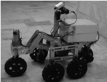
In this paper, an eective approach for kine-matic and dynamic modeling of high mobility Wheeled Mobile Robots (WMR) has been presented. As an example of these robots, the method has been applied to the CEDRA rescue robot, which is a complex, multibody mechanism [6] (Figure 1). The CEDRA rescue robot is one of several laboratory robots made
Figure 1.
CEDRA rescue robot.at the Center of Excellence in Design, Robotics and Automation (CEDRA).
The main structure of this robot is based on a shrimp-like mechanism, developed in EPFL [7], con-sisting of three main parts (see Figure 2): Main body, parallel bogies and front fork (a four-link mechanism): 1. Body: The main part of the robot, as a container for electronic boards, batteries, camera, navigation and victim detection instruments;
2. Parallel Bogies: This consists of two parallel four-link mechanisms mounted on each side of the main body, in order to stabilize it and increase the terrain adaptability of the robot;
3. Front Fork: A four-link mechanism mounted in front of the robot body that helps the robot in climbing obstacles.
Using a D-H coordinate denition, the forward kine-matics of the system have been evaluated in terms of joint angles and wheel rotations. Then, the parameters
Figure 2.
Three main parts of a shrimp mechanism.are separated, according to the actuated and sensed parameters, leading to the inverse kinematics of the rover.
Another demanding objective is to model the complicated dynamics of the CEDRA robot for use on uneven terrain. Since the robot is a 6-wheel rover with 2 steering commands and many linkages, Kane's approach has been preferred to other methods. Con-sidering really rough terrain modeling, the exibility of the tire and ground interaction has also been considered in the dynamic model.
KINEMATIC MODELING
The rst step in the modeling of robots is kinematic modeling. In this analysis, the motion of mass center will be determined in terms of known wheel motions and vice versa. Also, by setting a desired velocity for the mass center, one can derive the actuators velocity so that it can be utilized in the kinematic based control of the system.
The approach that will be discussed here is the basis for a kinematic analysis of WMRs on uneven terrain. At rst, a frame-work is constructed to express the position-orientation of the desired points, like wheel centers, contact points and joints. All these coordinates are dened using the Denavit-Hartenberg (D-H) method [8]. Then, by evaluating the trans-formation matrices between the robot reference frame and each wheel motion frame, the relative position of the motion frame, with respect to the robot center of mass, is derived. In order to obtain the robot forward kinematic, Jacobian matrices for each wheel are evaluated in a symbolic manner.
Coordinate Denition
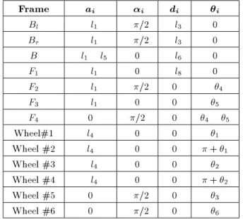
All the coordinate frames used in this article are right-hand coordinate systems. The robot reference frame is dened at the center of mass so that the x direction refers to forward motion and thez-axis heads upward. According to the D-H method [8], a coordinate frame is introduced on each joint. Since CEDRA is a 6-wheel robot, there are 6 separate open chains. Figures 3 and 4 depict the robot coordination.
A transformation matrix can be dened between two consequent frames, using the D-H parameters,ai,
i,di, i: i 1T
i=
2 6 6 4
ci sici sisi aici
si cici cisi aisi
0 si 1 ci 1 di
0 0 0 1
3 7 7
5; (1)
where:
ci= cosi; si= sini;
ci 1= cosi 1; si 1= sini 1:
Table 1 provides the D-H parameters corresponding to the coordinate frames in Figures 3 and 4.
Then, by cascading the transformation matrices in the chains, the position of each wheel is obtained in the body coordinate, named the robot reference frame. In fact, the transformation matrices are the augmented
Figure 3.
Body and front fork coordinates.Figure 4.
Bogie coordinates.Table 1.
D-H parameters for wheel center coordinate frames.Frame
ai i di iBl l1 =2 l3 0
Br l1 =2 l3 0
B l1 l5 0 l6 0
F 1
l
1 0
l
8 0
F 2
l 1
=2 0
4 F
3
l
1 0 0
5 F
4 0
=2 0
4
5
Wheel#1 l
4 0 0
1
Wheel #2 l
4 0 0
+ 1
Wheel #3 l
4 0 0
2
Wheel #4 l
4 0 0
+ 2
Wheel #5 0 =2 0
3
Wheel #6 0 =2 0
6
matrix of a 33 rotation matrix and a 31 translation (position) vector.
For example, for the transformation from the rover reference frame, R, to the wheel 1 axle frame, one has the following:
RT
1=
RTBlBlT
1: (3)
However, in order to capture the wheel motion, one needs two more coordinate frames. Two additional coordinate frames are dened for each wheel, i.e., contact frameCi and motion frame Mi, i = 1;;6. The contact coordinate frame,Ci, denes the location
of the wheel-terrain contact point. It is obtained by a rotation of the wheel axle coordinate frame about thez-axis, followed by a 90 degree rotation about the
x-axis. The z-axis of the Ci frame points away from
the contact point, as illustrated in Figure 5. The D-H parameters for theCiframes,i= 1;;6, are provided in Table 2.
The wheel motion frame, Mi, accounts for the
wheel roll and rotational slip. It is obtained by rotating about the Ci frame's z-axis a rotational slip
(i), translating along the negativez-axis by the wheel
radius (Rw) and, nally, translating along the x-axis
for wheel roll (Rw:i) on a virtual inclined surface, as
illustrated in Figure 5. Corresponding D-H parameters are provided in Table 3.
Now, one can write the transformation matrices for each wheel's motion coordinate frame (Mi), in
Figure 5.
Contact and motion frames.Table 2.
D-H parameters for contact coordinate frames.Frame
a ii
d i
i C
1 0
=2 0
1 1
C
2 0
=2 0
1 2
C
3 0
=2 0
2 3
C
4 0
=2 0
2 4
C
5 0
=2 0
5 C
6 0
=2 0
Table 3.
D-H parameters for motion coordinate frames.Frame
ai i di iM1 Rw:1 0 Rw 1
M 2 R w : 2 0 R w 2 M 3 R w : 3 0 R w 3 M 4 R w : 4 0 R w 4
M5 Rw:5 0 Rw 5
M6 Rw:6 0 Rw 6
terms of the rover's reference frame (R). The trans-formations for wheel 1 are as follows:
RTM
1=
RTBlBlT
1 1T
C1
C1T
M1: (4)
Forward Kinematics
In view of the fact that the inverse of the transforma-tion matrix is equal to the inverse chain transformatransforma-tion matrix, one has the following [4]:
RT_R=RTM
i
MiT_
R: (5)
In contrast with Tarokh et al. [4] who have substituted
i = 0, the absolute rotations of the wheels, i, will
disappear from these equations, meaning that there should not be any angular position in the velocity distribution. Tarokh et al. [4] have substitutedi = 0,
but, in fact, there should not be any angular position in the velocity distribution.
Using Z Y X Euler angles, (heading),
p (pitch) and r (roll), the derivative of the rover coordinate frame, RT_R, is found to have the following form:
RT_R=
2 6 6 4
0 _ p_ x_ _
0 r_ y_
_
p r_ 0 _z
0 0 0 1
3 7 7
5: (6)
The angles correspond to rotations about the rover's reference frame (i.e., about the z-axis, pabout the
y-axis andrabout thex-axis).
After factorization of the velocity components of joint angles in the right side of Equation 5 and extract-ing the velocity vector,v =
_
x y_ z_ _ p_ r_T , the Jacobian matrix for each wheel is derived as follows:
v=Jiq_i i= 1;;6: (7)
For instance, for wheel 1, one has the following:
v= 2 6 6 6 6 6 6 6 6 6 6 4
l4s(1) Rwc( 1)c(1) l2c( 1) l3+l4s(1)
l3c( 1)
0 Rws(1) l1c( 1) 0 +l4c(1+ 1)
l4c(1) Rws( 1)c(1) l2s( 1) l1+l4cs(1)
0 0 c( 1) 0
0 0 0 1
0 0 s( 1) 0
3 7 7 7 7 7 7 7 7 7 7 5 2 6 6 4 _ 1 _ 1 _ 1 _1 3 7 7
5: (8)
Inverse Kinematics
The actuated inverse solution is used by solving Equa-tion 7 for the actuated wheel velocities. The outputs of the trajectory tracking controller are generally the rover forward velocity and turning rate. So, _xdand _d
are introduced as the controller commands. Also, bogie angles _1 and _2 and front four-link angle _4 can be measured relative to the body. It is assumed that the path planning unit has provided a complete sense of the terrain prole (Z=f(X;Y)) and one has _1(i= 1::6) at the contact points. Moreover, the outputs of the inverse kinematics unit should be the angular velocity of the actuators, consisting of 6 wheel motors and 2 steering motors.
Because of the closed-link chains in the wheeled mobile robot, it is not necessary to actuate all of the wheel variables. To separate the actuated and unactu-ated wheel variables, the wheel kinematic equation is partitioned into two components, as follows [1]:
Eivd=Jaiq_ai+Juiq_ui; i= 1;;6: (9) As an example for the 1st wheel, one has the following:
2 6 6 6 6 6 6 4
1 0 l4s(1) l3 l4s(1)
0 0 0 0
0 0 l4c(1) l1 l4c(1)
0 1 0 0
0 0 0 1
0 0 0 0
3 7 7 7 7 7 7 5 2 6 6 4 _
x_d
d _ 1 _1 3 7 7 5 = 2 6 6 6 6 6 6 4
Rwc( 1)c(1)
Rws(1)
Rws( 1)c(1) 0 0 0 3 7 7 7 7 7 7 5 _ 1
+ 2 6 6 6 6 6 6 4
l2c( 1) 0 0 0 0
l3s( 1) l1c( 1)+l4c(1+ 1) 1 0 0 0
l2s( 1) 0 1 0 0
c( 1) 0 0 0 0
0 0 0 1 0
s( 1) 0 0 0 1
3 7 7 7 7 7 7 5 2
6 6 6 6 4 _
1 _
y
_
z
_
p
_
r
3 7 7 7 7 5
; (10)
where the left side refers to the controller commands and the known parameters,Jaiis the Jacobian of
actu-ated components andJuiis the Jacobian of unactuated
components.
Then, the actuated inverse solution is applied in [1], as follows:
_
qai=
JTai(Jui)Jai 1
JTai(Jui)Eivd; i=1;;6; (11) where:
(J) =J(JTJ) 1JT I: (12) By substituting and simplifying the above equations, the following is obtained:
_
1= _
xd l2_d l4sin(1) _1 (l3+l4sin(1)) _1
Rwcos( 1)cos(1)
;
_
2= _
xd l2_d+l4sin(1) _1 (l3 l4sin(1)) _2
Rwcos( 2)cos(2)
;
_
3= _
xd+l2_d l4sin(2) _2 (l3+l4sin(2)) _3
Rwcos( 3)cos(3)
;
_
4= _
xd+l2_d+l4sin(2) _2 (l3 l4sin(2)) _4
Rwcos( 4)cos(4)
;
_
5=
_
xd l6cos(3) _5
Rw(cos(3)cos( 5)cos(5) sin(3)sin(5))
;
_ 6
=
_ x d
+l 8
_ 4
(l 8
+l 9
sin( 4
)) _ 5 R
w (sin(
4
5
6 )sin(
6 )+cos (
4
5
6 ) cos (
6 )cos (
6 ))
: (13) As can be seen, the steering rate cannot be derived through this method, since it is coupled with the rotational slip.
Geometric Method for Steering Angles
Since steering and rotational slip cannot be distin-guished for steerable wheels, one cannot use the Ja-cobian approach for steering commands as is used for the wheel rotation velocities. Therefore, a geometric approach is used, which determines the desired instan-taneous steering angle.
Due to the fact that the 4 bogie wheels are nonsteerable, rotational slip plays an important role in the direction of the wheel center velocity during robot turning and each xed wheel determines the instantaneous turn center, as illustrated in Figure 6.
First,Rw_1 and _1 components are rewritten for xed wheels, such as wheel 1:
_
x1=Rw_1
= _xd l2_d l4sin(1) _1 (l3+l4sin(1)) _1 cos( 1)
;
(14) _
1= _1= _
d
cos( 1)
: (15)
Each non-steerable wheel independently determines an instantaneous turn radius and turn center location [4]:
ri = _x_ii; (16)
cturn i=
RTCiri~yCi; i= 1;;4: (17) For wheel 1, one obtains the following:
r1= _
xd l2_d l4sin(1) _1 (l3+l4sin(1)) _1 _
d ; (18)
Figure 6.
Coordinate frames for steering angle calculations.cturn 1 =
RTC
1r1~yC1 =
2 6 6 4
c( 1) 0 s( 1) l1+l4c(1)
0 1 0 l2
s( 1) 0 c( 1) l3 l4s(1)
0 0 0 1
3 7 7 5
2 6 6 4 0
r1 0 1 3 7 7 5
= 2 6 6 6 4
l1+l4cos(1) _
xd l2 _
d l4s (
1 )
_
1 (l
3 +l
4s (
1 ))
_ 1 _
d
+l2
l3 l4s(1) 1
3 7 7 7 5
: (19)
Here, there are four unique turn centers, which will be unied by an approximation method [4]:
cturnR= 14 4 X
i=1
cturni: (20)
Now, using a geometric approach, the steering angles will be found (see Figure 6). The vector, r, denes the turn center relative to the steering wheel contact coordinate frame. Then, this quantity is determined for each steerable wheel, as follows [4]:
ri=RT 1
Cicturn
R; i= 5;6; (21)
where,cturn
Ris the estimated turn center calculated in the previous section and RTCi is the transformation
matrix between the rover's reference frame and the wheel,i, contact frame. Since the steerable axis is the
z-axis, one is only concerned with the projection of r
in thex y plane.
The desired steering angle for steerable wheeliis, then;
i=atan2( sign(ryi)rxi;jryij); i= 5;6: (22)
KANE'S METHOD
Kane's method, developed in the 1980's, is the most recent approach to motion dynamic analysis [9]. This method has demonstrated conspicuous predominance over others, like Newton and Lagrange, in complex problems. In fact, the ecacy of this approach is related to the lower number of equations, closed forms of equations, ease of deriving the constraint forces and better implementation of the numerical solutions, especially in dealing with the multiplicity of masses in the system. It is also widely used in nonholonomic problems, since the Lagrange method cannot handle nonholonomic constraints easily.
Kane's method uses the same list of denitions for its concepts as the Newtonian method, but, in order to distinguish the new expressions, a word \generalized" appears as a prex to that concept. For a system with
n-Degrees Of Freedom (DOF) andm-generalized coor-dinates, \generalized speeds" are dened as follows:
ur=zr(q;t) +Xm
i=1
yri(q;t) _q1; (1< r < n); (23) where _qi is the time derivative of qand yri andzr are
functions ofqand timet. The word \speed" is to show the scalar nature of the parameter.
The number of generalized speeds is equal to the number of DOF. According to the denition of generalized speed and by solving the equation for _qi,
one has the following: _
qs=Zs(q;t) +Xn
i=1
Ysi(q;t) _ui; (1< s < m); (24)
where,ZsandYsiare functions ofqand timet.
Now, the partial linear velocity and the partial angular velocity of pointP are introduced, as follows:
~VPr = @~V@uPr; (25)
~!Br= @~!@uBr; (26)
VP and !B are the velocities of point P. Also, the
velocity of any point can be derived from the linear combination of partial velocities associated with that point:
~VP =~vP(q;t) +Xn
i=1
~VPiui; (27)
~!B= ~WB(q;t) +Xn
i=1
~!Biui: (28)
Like other methods based on the calculus of variation (such as the Lagrange method), here, the generalized forces are dened, which means the partial derivative of active forces or torques inserting energy to the system. These forces might be external or internal, like internal friction forces.
Fr=X
i=1
~Vir:~Ri+X
j=1
~!jr: ~Mj; (29)
~Ri(1i) is foractive forces and ~Mj(1j) is for active torques. In this approach, inertial terms are considered, due to the D'Alambert viewpoint of dynamic equations, and can be written as follows:
~
RB = mB~aB; (30)
~
By summation of these equations for all bodies, one obtains the following:
F
r =
X
i=1
~Vir:
~Ri+~!ir:
~Mi
: (32)
Equilibrium equations associated with the D'Alambert viewpoint will lead to Kane's equations and can be represented as:
F
r +Fr= 0: (33)
Kinematic Constraints
To get a better sense of the dynamic problem, the De-grees Of Freedom (DOF) and the required parameters for a determined conguration are discussed.
Consider the main body in 3D space with 6 DOF. Adding 3 angular freedoms in the bogies and front fork, 6 wheel rotations and 2 steering angles allow the rover to have 17 DOF in space. But, since it traverses on the ground, 6 motions will be conned and the total number of DOF will equal 11. In the condition of no longitudinal slip, 6 other DOF will be limited and the total DOF decreases to 5.
Here, a complete model of rover motion is to be developed, in which slipping and skidding (i.e., longi-tudinal and transversal slippage) will be considered.
To determine the robot conguration completely, 11 independent parameters should be assigned, which are chosen here to be _x, _y, _, _1::6, _3and _6(steering), as generalized speeds.
In order to nd the ground reaction force, a velocity is introduced at the center of each wheel. Therefore, the normal force and total friction force on the wheels can be derived.
Finally, the total number of generalized coordi-nates equals 35 and their rate of change will be:
_
q= "
_
1;2 |{z} Bogie
_
4 |{z} Fork
_
z p_ r V_ |{z}wx
6
Vwy
|{z} 6
Vwz
|{z} 6 _
x y_ _ _i
|{z} 6
_
3;6 |{z} Steering
#T
: (34)
Since the normal velocity of wheel centers relative to the ground is a virtual velocity, an additional set of generalized speeds is dened. If the terrain prole is dened asZ=f(X;Y), one will have the following:
uj =
2 4
Vwix
Vwiy
Vwiz 3 5:
rf; for : j= 1217: (35) As mentioned above, one needs to nd 18 constraints to conne 35 generalized coordinates to 17 generalized
Figure 7.
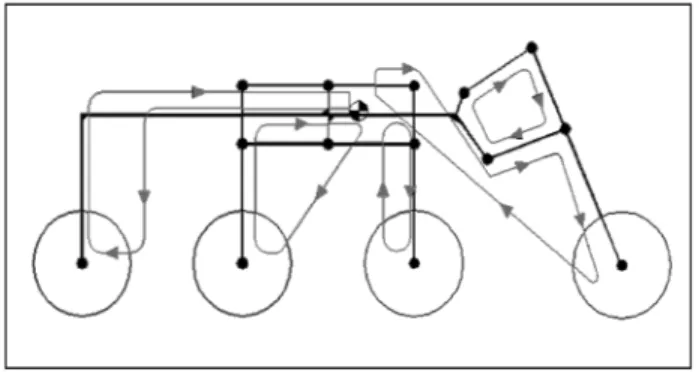
Closed-loop chains.speeds. Figure 7 illustrates the schematic 2D sketch of closed loop chains between the rover reference frame and wheels. The other bogie has not been shown here, so, there are six 3D constraints. _5 has been omitted from the generalized coordinates, hence, the relation between _4and _5 in the front fork is not considered in the constraints.
In the kinematic part, the velocities of the wheel centers have been dened in the rover reference frame,
R, using the D-H method described in the previous sections. For example, for wheel 1, one has a closed loop chain as follows:
Vw1 h
I33 ... 031 i
oTRRTw
1
0 0 0 1T =0;
(36) in which,oTRis the transformation matrix of the robot
reference frame, with respect to the global coordinate.
oTR=
2 6 6 6 6 6 6 4
c()c(p) c()s(p)s(r) c()s(p)c(r) x s()c(r) +s()c(r)
s()c(p) s()s(p)s(r) s()s(p)c(r) y
+c()c(r) c()s(r)
s(p) c(p)s(r) c(p)c(r) z
0 0 0 1
3 7 7 7 7 7 7 5
:
(37) Since Equation 36 presents 3 motion constraints, 18 constraint equations will be obtained by the closed-loop chains.
Now, the constraint equations need to be rear-ranged to construct a standard form of Equation 24. For this purpose, the generalized coordinates are fac-torized and, then, the denition of inputs are aug-mented, leading to a 3535 matrix.
2 6 4
A1835
: : : : : : : : : : : : : :
01718 ...I1717 3 7 5q_
351=
0118 ...u1 u2 u
17
;
(38) or:
A1(3535)(q) _q= 17 X
i=1
Biui;
BTi =h
01(17+i) ... 1 ... 01(17 i) i
; (39)
or: _
q=A 1 1 (q)
17 X
i=1
Biui=
17 X
i=1
Gi(351)ui:
DYNAMICAL ANALYSIS
In this section, a systematic procedure for the dynamic modeling and formulation of WMRs is presented for 3D motion on rough terrain. The analysis will be based on Kane's method. Here, an approach for extraction of Kane's items, like generalized inertial forces and generalized active forces, has been demonstrated. As an illustrative example, this method has been applied to the CEDRA rescue robot.
Inertial Forces
Since a distributed mass analysis is very demanding and does not seem to be reasonable in rover dynamics, 8 noticeable point masses are assumed consisting of 6 wheels, a front fork and a main body. The velocities of these masses will easily be evaluated using the D-H method explained in the previous section.
Vwj=h
I33 ... 031 i
oTRRTwj
0 0 0 1T
;
forj= 1::6; (40)
VFF =h
I33 ... 031 i
oTRRTf
4[xFF 0 zFF 1]
T;
(41)
VMB =h
I33 ... 031 i
oTRRTMB
xMB 0zMB 1T
;
(42) or:
Vmj =
Vmj335(q) _q 351= 17 X i=1
Vmj335Gi (351)
ui;
forj= 1::8: (43)
The partial velocities of the wheel centers can be expressed as:
~Vpr=@~V@urp ) ~Vrmj = [
Vmj335Gr
(351)]: (44)
Also, accelerations associated with point masses are found by the derivation of velocities, as follows:
amj = dtVd mj =17 X i=1 8 < :
Vmj335Gi (351)
_
ui+@[
Vmj335Gi (351)]
@q qu_ i
9 = ; = 17 X i=1 [
VmjGi] _ui+ 17 X i=1 17 X k=1 2 4@[
VmjGi]
@q Gk
3 5ukui:
(45) Furthermore, one needs to evaluate the angular velocity vectors of the wheels, the main body and the front fork:
!wj=oTrotation
R(33) 0 @ 2 4 _ r _ p _ 3 5+ 2 4 0 _ j 0 3 5 1
A; forj= 1::6; (46)
!FF =oTrotation
R(33) 0 @ 2 4 _ r _ p _ 3 5+ 2 4 0 _
4 _5 0
3 5
1
A; (47)
!MB =oTrotation
R(33) 2 4 _ r _ p _ 3
5; (48)
or:
!mj =
!mj335(q) _q 351= 17 X i=1 h
!mj335Gi (351)
i
ui;
forj= 1::8; (49)
where oTrotation
R(33) is the rotational part of
oTR and the
corresponding partial angular velocity will be:
~!rmj = [
!mj335Gr
(351)]; (50)
mj =d
dt!mj =
17 X
i=1 [
!mjGi]_ui
+ 17 X i=1 17 X k=1 " @[
!mjGi]
@q Gk
#
ukui: (51)
The generalized forces are derived by substituting the above parameters in Equations 30 to 32.
F 1 = 8 X j=1
mj(~V1mj:~a
mj) +Ij(!mj
1
mj)
Gravity Force
The partial velocities associated with each weight force exertion point are equal to the partial velocities of the center of gravity of the bodies. Also, the weight forces are simply described by:
~Fwj = m
jg 2 4 0 0 1 3
5: (53)
Motor Torques
Inserted energy to the system is provided by the motors; hence, the torque vector is dened as:
=
1 2 3 4 5 6 T
; (54)
and the angular velocities of these torques are:
!j = _
j ;_ j = 1; 2; 3; 4; 5;
!6 = _
6 :_ (55)
Now, by deningE in the form of:
Er=
h
!1
!2
!3
!4
!5
!6 i
TGr; (56)
the motor torques in dynamics modeling can be in-cluded.
Ground Force
An interaction force is exerted under each wheel that can be dened as:
Fgj = 2 4
Fxgj
Fygj
Fzgj
3
5: (57)
The velocity of the ground force action point is easily evaluated using the motion coordinate frame, after setting to zero.
Vcj=h
I33 ... 031 i
oTRRTmj
0 0 0 1T
= 2 4
Vxcj
Vycj
Vzcj
3 5 31 = 2 6 6 4 Vcjx Vcjy Vcjz 3 7 7 5q_=
17 X i=1 0 B B @ 2 6 6 4 Vcjx Vcjy Vcjz 3 7 7 5Gi
1 C C Au;
forj = 1::6; (58)
Vrcj=
2 6 6 4 Vcjx Vcjy Vcjz 3 7 7
5Gr: (59)
And, eventually, the generalized force associated with the contact points is:
Fgr= 6 X
j=1
Vrcj:~Fgj (60)
Kane Formulation
The closed form equation for the dynamics of the rover can be derived as follows:
17 X
i=1
Mri(q) _ui+ 17 X i=1 17 X j=1
Nri;j(q)uiuj+gWr(q) +Fgr(q; ~Fgj) =:Er(q); r= 1::17;
(61) where the coecients are:
Mr(q) =
8 X
j=1 (mj[
VCjA 1 1 ]:[
VCjA 1 1 ] +Ij[
!jA 1 1 ]:[
!jA 1 1 ]);
Nr(q) =
8 X
j=1 (mj[
VCjA 1 1 ]:@
[
VCjA 1 1 ]
@q
+Ij[
!jA 1 1 ]:@
[
!jA 1 1 ]
@q )A 1 1 ;
Wr(q) =
8 X
j=1
mj[
VCjA 1 1 ]:
2 4 0 0 1 3
5: (62)
The above equations are the closed form equations of motion for the CEDRA rover, consisting of 17 equations, 17 generalized speeds and 18 ground force components. Hence, one should nd 18 constraint equations. The dynamics of WMRs, in the presence of slip, do not usually have an analytical solution, since in non-slip conditions, a kinematic constraint restricts the rotational motion of the wheel and, in cases of slipping, a dynamic constraint relates the normal force with the friction force. Therefore, a decision tree is needed for the numerical solution. First, a rigid wheel on a rigid terrain is considered:
(I) Wheelj doesn't slip:
(1) Because of skidding, transversal friction force is equal to:
CFygj= sCFzgj; (63)
where, CFzgj and CFygj are the normal and
transversal ground reaction forces in the contact coordinate frame;
(2) It is assumed that wheels do not lose their contacts, so,
u12=u13= =u
(3) The longitudinal motion of each wheel is dependant on the wheel rotation.
Vxj=Rw_j; j = 1::6; (65)
where the longitudinal velocity is the pro-jection of Vwj in the contact frame x-axis
direction.
With these 18(= 3 6) extra con-straints, they can be solved simultaneously with Equation 61. At each time step, 35 equations with 35 unknowns are solved and all ground contact forces are determined. Now, assumption I should be checked for validity.
q
(CFxgj)2+ (CFgj
y )2
CFzgj s: (66) If Condition 66 doesn't hold for the obtained forces, this time step should be solved once again with assumption II.
(II) Wheelj slips:
(1) Friction force that is always in the direction of motion is, as follows:
Vxj
Vyj = CFxgj
CFygj: (67)
(2) Equation 64 is valid for this case too; (3) The dynamic constraint of contact force is:
q
(CFxgj)2+ (CFgj
y )2=CsFgj
z : (68)
Again, after solving 35 equations, one goes through the next time step. Now, in a more realistic approach, the ground exibility in the constraints is considered. The method does not change, except for the assumptions made in the previous section. Since the friction coecient changes its nature, Equa-tion 63 does not hold in this case.
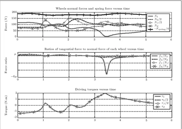
SIMULATION
The obtained equations can be used for various pur-poses, such as: Dynamics optimization, checking avail-able control strategies, inverse and forward dynamic simulation and comparison between various rovers. But, as far as there has been a focus on obtaining the equations themselves, only a simpler simulation is described. Due to the complexity of the 3D case, the simulation illustrated here will concentrate on the 2D vertical plane. There are several reasons for this 2D simulation. The mechanisms (like bogies and front
fork) move in parallel planes and there is no linkage and exibility in the 3rd dimension. Therefore, the rover dimensions are more eective and more meaningful in the planner analysis. Moreover, the rst step in the design of rovers is checking its capability of climbing over obstacles and this model has been used to develop climbing abilities through dynamical equations of motion. In simulation, the robot is forced to pass a bump generated by a function like \he (
x w )
2
", similar to the previous work [10]. The \h" is selected equal to \w" and about 2.25 times the wheel radius. It is assumed that all six wheels torques are equal. The above mentioned task has been applied to the robot and the results are shown in Figure 8. As can be seen, after a transient response, it will follow the same behavior as before. Consequently, the values of normal forces, friction forces and their ratios have changed.
CONCLUSIONS
A general frame-work for kinematic and dynamic analysis of rovers has been developed, consisting of forward and inverse kinematics in a control oriented approach and by deriving the dynamics equations based on Kane's method. The analysis has been applied to the CEDRA rescue robot as an illustrating example. In order to reach a desired velocity on rough terrain, the equations of the actuators' eort have been derived.
This work has mainly focused on the detailed steps of dynamic formulation rather than dynamic analysis of the CEDRA robot. However, future work is required to perform a more exact analysis of this robot and to extend the application of this method.
Based on D-H and Kane's methods, a systematic method for deriving equations of motion governing a rover has been presented. The method is very ecient for numerical purposes.
In addition, it has been shown that the method is capable of extracting exact symbolic equations for a rover with one of the most complicated mechanisms, including four closed chains. Also, it is capable of calculating constraint forces easily and handling them to generate traction control algorithms for high velocities over uneven terrain. Both the kinematics and kinetics are presented here and, also, this method oers an appropriate set of coordinates to fully and easily describe rover conguration. This method, which can be used in the selection of state variables, extraction of rate equations and, also, in meaningful descriptions of various terms of equations, is very useful and novel in its own right. It must be mentioned that for 3-dimensional motion, governing equations are highly complicated and seem not to be handled and solved symbolically. Hence, a numerical method may be used to deal with the problem.
Figure 8.
Simulation results for ground forces and motor torques vs. time.NOMENCLATURE
BTA transformation matrix fromAtoB
ai;i anddi joint parameters in D-H notation
i joint variable in D-H notation
Bl left bogie coordinate frame
Br right bogie coordinate frame
B back coordinate frame
Fi ith front coordinate frame
Ci ith contact coordinate frame
Mi ith motion coordinate frame
Rw wheel radius
i ground slope underith wheel
i ith wheel absolute rotation
i angular slip
_
x;y;_ z_ robot velocities in direction of body coordinate frame
;r;p robot yaw, roll and pitch angles _
xd desired longitudinal velocity
v velocity vector
J Jacobian matrix
qi ith wheel parameter vector
Jai ith wheel actuated Jacobian matrix
Jui ith wheel unactuated Jacobian matrix
qai ith wheel actuated parameter vector
qui ith wheel unactuated parameter vector
ci instantaneous turn center for ith
unsteerable wheel
ri turn radius forith unsteerable wheel
Fr sum of generalized non-inertia forces
u generalized speeds column vector _
q rate of change of generalized coordinates
g gravitational acceleration
N wheel normal force column vector _
d desired yaw rate
cturnR instantaneous robot turn center
mj mass ofjth part
~Vrmj rth partial mass center velocity ofjth
part
~!rmj rth partial mass center angular velocity
ofjth part
~Vmj mass center velocity ofjth part
~!mj mass center angular velocity of jth
part
~mj mass center angular acceleration ofjth
part
IB moment of inertia of bodyB around
the CM
F
r sum of generalized inertia forces
wheels torque column vector
!i
corresponding angular velocity toith applied torque
_
u rate of change of generalized speeds
Fxgj;Fygj;Fzgj components of ground reaction in
global coordinate frame
CFxgj;CFygj;CFzgjcomponents of ground reaction force in
the contact coordinate frame
REFERENCES
1. Muir, P.F. and Neuman, C.P. \Kinematic modeling of wheeled mobile robots",J. Robotics Systems,
4
(2), pp 281-340 (1987).2. Chottiner, J.E. \Simulation of a six-wheeled martain rover called the rocker-bogie", M.S. Thesis, Ohio State University, Columbus, Ohio, USA (1992).
3. Linderman, R. and Eisen, H. \Mobility analysis, simulation and scale model testing for the design of wheeled planetary rovers", In Missions Technologies
and Design of Planetary Mobile Vehicle, Toulouse, France, pp 531-537 (1992).
4. Tarokh, M., McDermott, G., Hayati, S. and Hung, J. \Kinematic modeling of a high mobility Mars rover", IEEE Conf. on Robotics and Automation, Detroit, MI, (May 1999).
5. Tai, M. \Modeling of wheeled mobile robot on rough terrain",ASME International Mechanical Engineering Congress, Washington, D.C., USA (2003).
6. Meghdari, A., Pishkenari, H.N., Gaskarimahalle, A.L., Mahboobi, S.H. and Karimi, R. \Optimal design and fabrication of CEDRA rescue robot using genetic al-gorithm", CD-ROM Proceeding of the ASME-DETC-2004 (MR-57190), Salt Lake City, Utah (2004). 7. Siegwart, R., Lamon, P., Estier, T., Lauria, M. and
Piguet, R. \Innovative design for wheeled locomotion in rough terrain", J. of Robotics and Autonomous Systems,
40
(3), pp 151-162 (2002).8. Craig, J.J., Introduction to Robotics: Mechanics and Control, 2nd Ed., Addison-Wesley Pub., USA (1989). 9. Kane, T.R. and Levinson, D.A., Dynamics: Theory
and Applications, McGraw-Hill (1985).
10. Meghdari, A., Karimi, R., Pishkenari, H.L., Gaskarimahalle, A.L. and Mahboobi, S.H. \An eec-tive approach for dynamic analysis of rovers", Robot-ica,