Quintic Spline Solution of Boundary Value Problems in the Plate De ection Theory

Electrical Engineering Vol. 16, No. 1, pp. 53{59

c

Sharif University of Technology, June 2009 Research Note

Quintic Spline Solution of Boundary Value

Problems in the Plate Deection Theory

J. Rashidinia

1;

_{, R. Mohammadi}

1

_{and R. Jalilian}

1

Abstract. In this paper, Quintic spline in o-step points is used for the solution of fourth-order boundary value problems. Spline relations and boundary formulas are developed and the convergence analysis of the given method is investigated. Numerical illustrations are given to show the applicability and eciency of our method.

Keywords: Fourth-order ordinary dierential equation; Quintic spline; O-step points; Convergence analysis; Monotone matrix.

INTRODUCTION

We consider the fourth-order boundary value problems of the form:

u(4)_{(x) + f(x)u(x) = g(x); a x b; (1)}

subject to the following boundary conditions:

u(a) = A1; u(b) = A2;

u00_{(a) = B}

1; u00(b) = B2; (2)

where f(x) and g(x) are continuous on [a; b] and Ai, Bi,

i = 1; 2 are real nite constants. Such types of fourth-order boundary value problems arise frequently in the plate deection theory [1]. The analytical solution of the Problem in Equation 1 for the arbitrary choice of f(x) and g(x) cannot be determined [1-5]. We assume that u(x) is suciently dierentiable and that a unique solution of the problem in Equation 1 exists [2,3,6].

Further discussions of fourth-order boundary value problems are given in [1-3,7]. Usmani [1] dis-cussed the existence and uniqueness solutions of such problems when subjected to the following boundary

1. School of Mathematics, Iran University of Science and Tech-nology, Tehran, P.O. Box 16846 13114, Iran.

*. Corresponding author. E-mail: [email protected] Received 31 July 2007; received in revised form 24 October 2007; accepted 26 February 2008

conditions:

u(a) = A1; u(b) = A2;

u0_{(a) = B}

1; u0(b) = B2:

Sixth order methods for solving this problem were used by Usmani [2,3]. Methods of order two and four, based on quintic and sextic splines, were developed by Usmani [4,5]. Later, Usmani [6] used quartic splines for the numerical solution of fourth-order boundary value problems. Rashidinia [8] and Usmani et al. [9] derived the quintic spline and non-polynomial quintic spline methods for the solution of linear fourth-order boundary value problems. But all the derived methods use nodal points; only in [6] a quartic spline with o-step points is used.

In this paper, rst a direct method based on the quintic spline for fourth-order boundary value problems (Equation 1) is presented. Our aim is to approximate u(x) satisfying (Equation 1) by using quintic spline functions, 2 C4_{[a; b]. This approach will employ}

consistency relations at midknot.

Then, the quintic spline formulation is derived for the numerical solution of Equations 1 and 2. Following that to retain the bandwidth of the coecient matrix of the system as ve, we develop the end conditions of O(h6_{). Subsequently, convergence analysis is proved}

so that the matrix associated with the system of linear equations that arises is not assumed to be monotone, as often believed in the post. Finally, the numerical

evidence is included to demonstrate the eciency of the presented method.

QUINTIC SPLINE FUNCTION

We consider a uniform mesh, , with nodal points, xi

on [a; b] such that:

: a = x0< x1

2 < x32 < < xN 12 < xN = b;

where x_i 1

2 = a+(i

1

2)h, i = 1; 2; ; N and h = b aN .

Also, we denote a function value, u(xi) by ui.

Denition

A quintic spline function, Si(x), interpolating to a

function u(x) on [a; b] is dened as following:

1. In each subinterval, [xi; xi+1], Si(x) is a polynomial

of, at most, degree ve;

2. The rst-fourth derivatives of Si(x) are continuous

on [a; b];

3. Si(xi) = u(xi), i = 0(1)N.

The spline function, Si(x), for x 2 [xi; xi+1], is dened

by:

Si(x) = 5

X

k=0

a(k)_i (x xi)k; i = 0; 1; 2; ; N; (3)

where a(k)_i , k = 0; 1; ; 5 are constants to be deter-mined.

We further require that the values of the rst-, se-cond-, third- and fourth-order derivatives are the same for the pair of segments that join at each point (xi; ui).

To derive an expression for the coecients of Equation 3, in terms of u_i 1

2, ui+12, Mi 21, Mi+12, Fi 12

and F_i+1

2, we rst denote:

(i) Si(xi 1

2) = ui 12;

(ii) Si(xi+1

2) = ui+12;

(iii) S00 i(xi 1

2) = Mi 12;

(iv) S00 i(xi+1

2) = Mi+12;

(v) S_i(4)(x_i 1

2) = Fi 12;

(vi) S(4)_i (x_i+1

2) = Fi+12: (4)

From algebraic manipulation, we get the following expression:

a(0)_i =₇₆₈1 h5h4_F i 1

2 + Fi+12

48h2_M i 1

2 + Mi+12

+384u_i 1 2 + ui+12

i ;

a(1)_i =_5760h1 h7h4_F i+1

2 Fi 12

+ 240h2_M i 1

2 Mi+12

+5760u_i+1 2 ui 12

i ;

a(2)_i =₃₂1 h h2_F i 1

2 + Fi+12

+8M_i 1

2 + Mi+12

i ;

a(3)_i =_144h1 hh2_F i 1

2 Fi+12

+24M_i+1

2 Mi 12

i ;

a(4)_i =₄₈1 F_i 1

2 + Fi+12

;

a(5)_i =_120h1 F_i+1

2 + Fi 12

;

where i = 0; 1; 2; ; N. The continuity of the rst derivative implies:

M_i 3

2 + 22Mi 12 + Mi+12

= ₂₄₀h2 (7F_i 3

2 254Fi 12 + 7Fi+12)

+24_h2(u_i 3

2 2ui 12 + ui+12);

i = 2(1)N 1; (5)

and the continuity of the third derivative yields: M_i 3

2 2Mi 12 + Mi+12

= h₂₄2(F_i 3

2 + 22Fi 12 + Fi+12);

i = 2(1)N 1: (6)

Subtracting Equation 6 from Equation 5 and dividing it by 24, we obtain:

M_i 1 2 =

1 h2(ui 3

2 2ui 12 + ui+12)

h2

1920(Fi 32 + 158Fi 12 + Fi+12): (7)

Elimination of Mi's between Equations 6 and 7 leads

to the following useful relation: u_i 5

2 4ui 32 + 6ui 21 4ui+12+ ui+32

=₁₉₂₀h4 (F_i 5

2 + 236Fi 32 + 1446Fi 12

+ 236F_i+1

2 + Fi+32);

i = 3(1)N 2: (8)

NUMERICAL METHOD

Now, we consider Equation 1 subject to boundary con-ditions (Equation 2). We discretize the given system in Equation 1 at the grid points, xi, i = 3; 4; ; N 2,

and use the spline relation (Equation 8). We obtain the (N 4) linear algebraic equation in the (N) unknowns, ui 1

2, i = 1; 2; ; N, as:

1 +₁₉₂₀1 h4_f i 5

2

! u_i 5

2

+

4 + ₁₉₂₀236 h4_f i 3

2

ui 3

2

+

6 + 1446 360 fi 12

h4_u

i 1 2

+

4 + ₁₉₂₀236 h4_f i+1

2

u_i+1

2

+

1 + ₁₉₂₀1 h4_f i+3

2

u_i+3

2

= h4

1920(gi 52 + 236gi 32 + 1446gi 12

+ 236g_i+1

2 + gi+32); i = 3(1)N 2; (9)

where fi= f(xi) and gi= g(xi).

To obtain the unique solution of the above sys-tems, we need four more equations. By using a Taylor series and the method of undetermined coecients, the boundary formulas associated with boundary condi-tions (Equation 2) can be determined as follows:

a0u0+ a1u1

2 + a2u32 + a3u52 + ch

2_u00 0

+ h4h_b 1u(4)1

2 + b2u

(4)

3 2 + b3u

(4)

5 2

i

+ t1= 0; (10)

a0

0u0+ a01u1 2 + a

0 2u3

2 + a

0 3u5

2 + a

0 4u7

2 + c

0_h2_u00 0

+ h4h_b0 1u(4)1

2 + b

0 2u(4)3

2 + b

0 3u(4)5

2 + b

0 4u(4)7

2

i

+ t2= 0; (11)

and: a0

0uN + a01uN 1 2 + a

0

2uN 3 2 + a

0

3uN 5 2

+ a0 4uN 7

2 + c 0

h2_u00 N + h4

h b0

1u(4)N 1 2

+b0 2u(4)N 3

2 + b 0

3u(4)N 5 2 + b

0

4u(4)N 7 2

i

+ tN 1= 0; (12)

a

0uN + a1uN 1 2 + a

2uN 3

2 + a

3uN 5

2 + c

_h2_u00 N

+ h4h_b 1u(4)_N 1

2 + b

2u(4)_N 3

2 + b

3u(4)_N 5

2

i

+ tN = 0; (13)

In order that t1, t2, tN 1 and tN are O(h6), we nd

that:

(a0; a1; a2; a3; c) = (a0; a1; a2; a3; c)

=

6; 10; 5; 1;5₄

;

(b1; b2; b3) = (b1; b2; b3) =

383 960; 383 1920; 1 1920 ; (a0

0; a01; a02; a03; a04; c0) = (a

0

0; a

0

1; a

0

2; a

0

3; a

0

4; c

0

)

=

2; 5; 6; 4; 1;1₄

;

(b0

1; b02; b03; b04) = (b

0

1; b

0

2; b

0

3; b

0 4) = 383 1920; 113 192; 33 160; 1 1920 :

From the above relations, we obtain the following equations:

10 +383 960h4f12

! u1

2 +

5 +383 360h4f32

u3

2

+

1 + ₁₉₂₀1 h4_f5

2

u5

2 = 6u0

5 4h2u000

+₁₉₂₀h4 h766g1

2 + 383g32 + g52

i

+₁₁₅₂₀181 h6_u(6)₍

5 + ₁₉₂₀383 h4_f1 2 ! u1 2+

6 + 113₁₉₂h4_f3

2 u3 2 +

4 + ₁₆₀33h4_f5

2

u5

2 +

1 + ₁₉₂₀1 h4_f7

2

u7

2

= 2u0 1₄h2u000+ h 4

1920 h

383g1

2 + 1130g32

+396g5 2 + g72

i

+₁₁₅₂₀497 h6_u(6)₍

1) + O(h7);

i = 2; (15)

and:

1 + ₁₉₂₀1 h4_f N 7

2

! u_N 7

2

+

4 +₁₆₀33 h4_f N 5

2

u_N 5

2

+

6 + 113₁₉₂h4_f N 3

2

u_N 3

2

+

5+ 383

1920h4fN 12

u_N 1

2= 2uN

1 4h2u00N

+₁₉₂₀h4 hg_N 7

2+396gN 52+1130gN32+383gN 12

i

+₁₁₅₂₀497 h6_u(6)₍

N 1) + O(h7); i = N 1;

(16)

1 + ₁₉₂₀1 h4_f N 5

2

! u_N 5

2

+

5 + 38

1920h4fN 32

u_N 3

2

+

10 +383

960h4fN 12

u_N 1

2 = 6uN

5 4h2u00N

+₁₉₂₀h4 hg_N 5

2 + 383gN 32 + 766gN 12

i

+₁₁₅₂₀181 h6_u(6)₍

N) + O(h7); i = N: (17)

The scheme of Equation 9 along with boundary for-mulae (Equations 14, 15, 16 and 17) yields the ve diagonal linear system of order N N and may be written in matrix form as:

AU = C + T; (18)

AU = C; (19)

AE = T; (20)

where U = (ui 1

2), U =

ui 1

2

, T = ti 1 2

and E = e_i 1

2

=u_i 1 2 ui 12

for i = 1(1)N are N-dimensional column vectors.

Matrix A can be denoted by A = A0+ h4BF ,

where:

A0=

0 B B B B B B B B B B B B B B B @

10 5 1

5 6 4 1

1 4 6 4 1

... ... ... ... ... ... ... ... ... ...

... ... ... ... ...

1 4 6 4 1

1 4 6 5

1 5 10

1 C C C C C C C C C C C C C C C A

= P2_;

P is a monotone three diagonal matrix dened by:

pij =

8 > > > < > > > :

3 i = j = 1; N;

2 i = j = 2; 3; ; N 1; 1 ji jj = 1;

0 otherwise:

(21)

Matrix B is dened by:

B = ₁₉₂₀1

0 B B B B B B B B B B B B B B B @

766 383 1

383 1130 396 1

1 236 1446 236 1

... ... ... ... ... ... ... ... ... ...

... ... ... ... ... 1 236 1446 236 1

1 56 246 383

1 56 245

1 C C C C C C C C C C C C C C C A

C = [c1

2; c32; ; cN 12]

T _{given by:}

c1 2 = 6A1

5

4h2B1+ h4

1920(766g12 + 383g32 + g52);

c3

2 = 2A1

1 4h2B1

+₁₉₂₀h4 (383g1

2 + 1130g32 + 396g52 + g72);

c_i 1

2 = 0; i = 3(1)N 2;

c_N 3

2 = 2A2

1

4h2B2+ h4

1920(gN 7

2 + 396gN 52

+ 1130g_N 3

2 + 383gN 12);

c_N 1 2 = 6A2

5 4h2B2

+₁₉₂₀h4 (g_N 5

2 + 383gN 32 + 766gN 12):

The above system in Equation 18 can be solved by any direct or iterative methods.

CONVERGENCE ANALYSIS

Here, we investigate the convergence analysis of the given method. Here, ei is the discretization error and

ti is the local truncation error dened by:

ti=

8 > > > > > > < > > > > > > :

181

11520h6u(6)(1); i = 1 497

11520h6u(6)(2); i = 2; 1

24h6u(6)(i); i = 3(1)N 2; 497

11520h6u(8)(N 1); i = N 1; 181

11520h6u(8)(N); i = N;

x0< 1< x1 2;

x0< 2< x1 2;

x_i 1

2 < i< xi+12;

x_N 1

2 < N 1< xN;

x_N 1

2 < N < xN:

(22)

Theorem 1

Let u(x) be the exact solution of the boundary value problem in Equation 1 and u_i 1

2, i = 1; 2; ; N be the

numerical solution obtained by the dierence scheme (Equation 19). Then:

kEk1= O(h2);

provided h4_{jf(x)j < 1.}

Proof

We can write error Equation 20 in the following form: E = A 1_{T = [A}

0+ h4BF ] 1T

= [I + h4_A 1

0 BF ] 1A01T;

kEk1 kA 1k1kT k1

k[I + h4_A 1

0 BF ] 1k1kA01k1kT k1;

kEk1 kA

1

0 k1kT k1

1 h4_{kAk1kBk1kF k1}; (23)

provided that h4_kAk

1kBk1kF k1< 1.

For our numerical procedure based on Equa-tions 9, 14 to 17 we have B = IN, a unit matrix, thus

kBk1= 1.

Following [6], we have:

kA 1

0 k1 5(b a)

4_{+ 10(b a)}2_h2_{+ 9h}4

384h4 : (24)

Also, we have:

kT k1₁₁₅₂₀497 h6M6; (25)

where M6= maxju(6)()j, a b.

Substituting kA 1

0 k1, kBk1 and kT k1 from

Rations 23 and simplifying we obtain:

kEk1 497M6h

2

11520(384 jf(x)j) = O(h2); (26) where = [5(b a)4_{+ 10(b a)}2_h2_{+ 9h}4_{], provided}

that:

jf(x)j < 384 (b a)4_{(5 +} 10

N2 +_N94)

:

Consequently, it follows that the prescribed numerical method is a second-order convergent process. This completes the proof of Theorem 1.

NUMERICAL ILLUSTRATIONS

To illustrate the applicability and eectiveness of our method and also to compare our results with existing methods, we consider the following fourth-order bound-ary value problems. These problems have been solved by the presented method with step lengths h = 2 m_,

m = 2; 3; ; 8, and the maximum absolute errors in numerical solutions are listed in Tables 1 to 3. The computed results veried that, by reducing the step size from h to h=2, the observed errors are approximately reduced by a factor (1

2)2verifying the theoretical order

of the presented method. We also compared our results with the second-order methods in references [5,6,8-10].

Table 1. The maximum absolute errors in the solution of Problem 1.

h Our Method Order

1

4 4.23( 4)

1

8 3.89( 5) 3:44

1

16 2.02( 5)

1

32 5.74( 6) 1:81

1

64 1.47( 6)

1

128 3.71( 7) 1:98

Problem 1

Consider the linear BVP in [7]:

u4_{(x) u(x) = 4e}x_{; 0 < x < 1;}

u(0) = 1; u00_{(0) = 3;}

u(1) = 2e; u00_{(1) = 4e:}

The theoretical solution for this problem is:

u(x) = (1 + x)ex_:

This problem has been solved with dierent values of h = 1

4; ;1281 and the maximum absolute errors in

the solutions are tabulated in Table 1.

Problem 2

Consider the following linear BVP from [5,6,8,9]: u4_{(x) + xu(x) = (8 + 7x + x}3_)ex_{; 0 < x < 1;}

u(0) = 0; u00_{(0) = 0;}

u(1) = 0; u00_{(1) = 4e:}

The theoretical solution for this problem is: u(x) = x(1 x)ex_:

We applied our method and compared the results with those obtained in the quintic spline method at grid points [5,8], the quartic spline method at o-step points [6] and the nite dierence method [9]. The results in Table 2 show that our method is giving better accuracy.

Problem 3

Consider the following linear BVP from [5,6,8,10]: u4_{(x) xu(x) = (11 + 9x + x}2 _x3_)ex_;

1 < x < 1;

u( 1) = 0; u00_{( 1) =} 2

e; u(1) = 0; u00_{(1) = 6e:}

Table 2. The maximum absolute errors in the solution of Problem 2.

h Our Method In [5] In [6] In [8] In [9]

1

4 1:54( 3) 3:51( 3) 1:61( 3) | 7:16( 3)

1

8 1:89( 4) 8:67( 4) 4:24( 4) 1:74( 3) 1:74( 3)

1

16 9:17( 5) 2:16( 4) 1:08( 4) 4:15( 4) 4:33( 4)

1

32 2:59( 5) 5:40( 5) 2:70( 5) 1:07( 4) 1:08( 4)

1

64 6:68( 6) 1:35( 5) 6:75( 6) | 2:70( 5)

1

128 1:68( 6) | 1:69( 6) | 6:75( 6)

1

256 4:23( 7) | 4:13( 7) | |

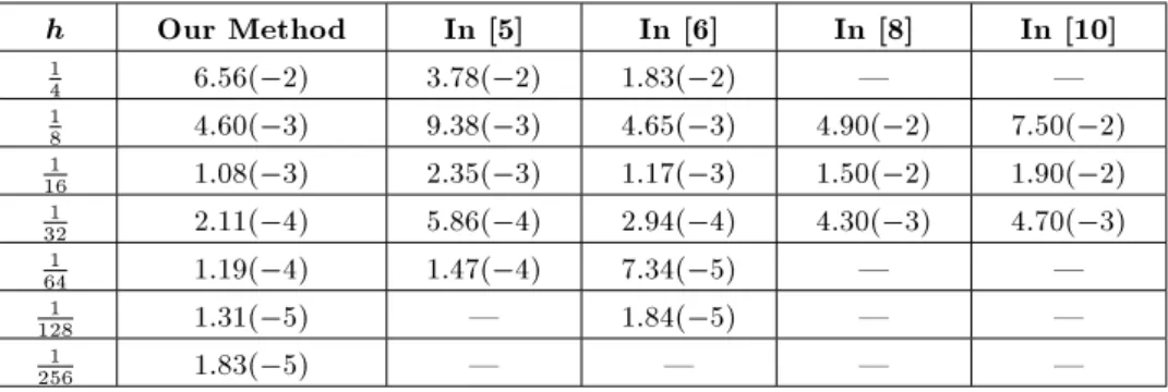
Table 3. The maximum absolute errors in the solution of Problem 3.

h Our Method In [5] In [6] In [8] In [10]

1

4 6:56( 2) 3:78( 2) 1:83( 2) | |

1

8 4:60( 3) 9:38( 3) 4:65( 3) 4:90( 2) 7:50( 2)

1

16 1:08( 3) 2:35( 3) 1:17( 3) 1:50( 2) 1:90( 2)

1

32 2:11( 4) 5:86( 4) 2:94( 4) 4:30( 3) 4:70( 3)

1

64 1:19( 4) 1:47( 4) 7:34( 5) | |

1

128 1:31( 5) | 1:84( 5) | |

1

The theoretical solution for this problem is: u(x) = (1 x2_)ex_:

We solved this problem by our method and compared our results with the quintic spline method at grid points [5,8], the quartic spline method at o-step points [6] and the nite dierence method [10]. The maximum absolute error in the solution of problem 3 is tabulated in Table 3, showing that the error in the solution of our method is less than in the methods in [5,6,8,10].

CONCLUSION

As we expected, the numerical results do conrm the second order of approximation. The maximum absolute errors in the solution of the fourth-order two-point boundary value problems given by our method are smaller than the errors in the methods in [5,6,8-10]. Moreover, we found that the developed quintic spline, using the o-step point, gives more accurate results in comparison with the quintic spline used in grid points.

ACKNOWLEDGMENT

The authors would like to thank the referees for their valuable suggestions and comments.

REFERENCES

1. Usmani, R.A. \Discrete methods for boundary value problems with applications in plate deection theory", J. Appl. Math. Phys., 30, pp. 87-99 (1979).

2. Usmani, R.A. \On the the numerical integration of a boundary value problem involving a fourth order linear dierential equations", BIT, 17, pp. 227-234 (1977). 3. Usmani, R.A. \An O(h6_{) nite dierence analogue for}

the solution of some dierential equations occurring in plate-deection theory", J. Inst. Maths. Applics, 20, pp. 331-333 (1977).

4. Usmani, R.A. \Smooth spline approximations for the solution of a boundary value problem with engineering applications", J. Comput. Appl. Math., 6(2), pp. 93-98 (1980).

5. Usmani, R.A. and Warsi, S.A. \Smooth spline solu-tions for boundary value problems in plate deection theory", Comput. Math. Appl., 6, pp. 205-211 (1980). 6. Usmani, R.A. \The use of quartic splines in the numerical solution of a fourth-order boundary-value problem", J. Comput. Appl. Math, 44, pp. 187-199 (1992).

7. Agarwall, R.P. \Boundary value problems for high ordinary dierential equations", World Scientic, Sin-gapore.

8. Rashidinia, J. \Direct methods for solution of a lin-ear fourth-order two-point boundary value problem", Intern. J. Eng. Sci., 13, pp. 37-48 (2002).

9. Usmani, R.A. and Marsden, M.J. \Numerical solution of some ordinary dierential equations occurring in plate deection theory", J. Eng. Math., 9(1), pp. 1-10 (1975).

10. Chawla, M.M. and Katti, C.P. \Finite dierence meth-ods for two-point boundary value problems involving high order dierential equations", BIT, 19, pp. 27-33 (1979).