Realised Volatility Forecasting: A Genetic
Programming Approach
Zheng Yin
Complex Adaptive SystemsLaboratory and School of Business University College Dublin
Dublin, Ireland Email:
Anthony Brabazon
Complex Adaptive SystemsLaboratory and School of Business University College Dublin
Dublin, Ireland Email:
Conall O’Sullivan
School of Business University College DublinDublin, Ireland Email:
Michael O’Neill
Complex Adaptive SystemsLaboratory and School of Business University College Dublin
Dublin, Ireland Email: [email protected]
Abstract—Forecasting daily returns volatility is crucial in finance. Traditionally, volatility is modelled using a time-series of lagged information only, an approach which is in essence atheoretical. Although the relationship of market conditions and volatility has been studied for decades, we still lack a clear theo-retical framework to allow us to forecast volatility, despite having many plausible explanatory variables. This setting of a data-rich but theory-poor environment suggests a useful role for powerful model induction methodologies such as Genetic Programming. This study forecasts one-day ahead realised volatility (RV) using a GP methodology that incorporates information on market conditions including trading volume, number of transactions, bid-ask spread, average trading duration and implied volatility. The forecasting result from GP is found to be significantly better than that of the benchmark model from the traditional finance literature, the heterogeneous autoregressive model (HAR).
I. INTRODUCTION
Volatility is an important concept in finance and has different implications depending on the perspective of the user. From an investment perspective, volatility is a measure of the degree to which returns tend to fluctuate. Traders would like to capture the volatility caused by positive returns, whereas in contrast, risk management is more concerned about the volatility caused by negative returns. Volatility is a key element in the pricing of derivatives, and is also a key input to the regulatory capital requirements from The Second Basel Accords.1 Hence, many stakeholders have an interest in being able to model and predict volatility.
In a conventional volatility model, volatility is a latent variable. The termrealised volatilitycan be broadly defined as the sum of intraday squared returns, measured at short intervals [1]. Such a volatility estimator has been shown to provide an accurate estimate of the latent process that defines volatility [2] and therefore, through realised volatility estimation, the latent volatility process is theoretically observable from past returns.
1Basel II are recommendations on banking laws and regulations issued by
the Basel Committee on Banking Supervision.
Genetic Programming’s (GP) model induction capability has been previously applied for volatility modelling and has achieved good results [5], [7], [8], [9] and [11]. However, there are still some important questions which have not been addressed. Market conditions have been documented as important volatility indicators and have been shown to have a high correlation with volatility in a number of studies. A sample of these studies include [12] which examined the relationship between trading volume and volatility, [13] examined the relationship between the number of transactions and volatility, [14] examined the relationship between price range and volatility, [35] examined the relationship between interest rates and volatility, [16] examined the relationship between implied volatility and volatility and [17] examined the relationship between the bid-ask spread and volatility. A better volatility forecast is expected when these market conditions are taken into the model as inputs, and this is the approach we take in this study.
In this paper, realised volatility (RV) is calculated using data drawn from one year of FTSE 100 index futures returns, sampled at a minute interval. It is well known that a five-minute sampling interval provides a good trade-off between accuracy, which is theoretically optimised using the highest possible frequency, and microstructure noise that can arise through the bid-ask bounce, asynchronous trading, infrequent trading and price discreteness, among other factors [18]. The calculated realised volatility is modelled directly using GP and the one-day-ahead RV is forecasted. Forecasting results from GP are compared with those from a benchmark HAR model which is drawn from the finance literature.
A. Structure of Paper
The remainder of this contribution is organized as follows. Section II provides some background on volatility modelling and provides the motivation for applying Genetic Program-ming to RV forecasting. Section III describes the data used in this study. The forecasting results are provided in Section IV and finally, conclusions and opportunities for future work are
discussed in Section V.
II. OVERVIEW OFVOLATILITYMODELLING
In this section we overview three key items. Initially, we provide an introduction to the concept of realised volatility. Then we briefly introduce current state-of-the-art approaches for the forecasting of realised volatility. Finally, we provide the motivation for the approach adopted in this paper, genetic programming.
A. Realised Volatility
Under the concept of RV, returns are assumed to be generated by the stochastic differential equation (Eq. 1), which is a continuous-time stochastic process over a given time period. The time period is divided into i equally-spaced adjacent intervals and the quadratic variation is defined as the limit of the sum of squared returns over these intervals, as the length of the sampling intervals goes to zero, where ti andti−1 are
adjacent intervals (Eq. 2). This limit is well-defined in the case of the logarithm price processp(t), which is a semi-martingale. In the general semi-martingale case, assuming some (mild) restrictions on the types of leverage, the quadratic variation is an unbiased estimator of the integrated variance,!0Tσ2(t)dt,
and the square root of the quadratic variation is called realised volatility.
dp(t) =σ(t)dW(t) (1)
lim
i−→∞(
"
i
(p(ti)−p(ti−1))2) (2)
Realised volatility can be used to measure the interdaily volatility by summing up the intraday squared returns at short intervals, such as five or fifteen-minute intervals [20]. This concept is very important to volatility modelling. It has been pointed out in [19] that the standard volatility models used for forecasting at the daily level can not readily accommodate the information in intraday data. The models specified directly for intraday data generally fail to capture the longer interdaily volatility movements sufficiently well. In contrast, using RV allows us to model volatility using relatively high frequency data, and also permits capture of stylised facts concerning interday volatility [19], [20].
In an ideal world, the quadratic variation from shorter intervals (as per Eq. 2) is always closer to the integrated volatility than the one calculated using longer intervals. How-ever, returns measured at intervals shorter than five minutes are plagued by spurious serial correlation caused by various market microstructure effects including asynchronous trading, discrete price observations, intraday periodic volatility pattern and the bid-ask bounce [2].
In reality, prices are observed at discrete and irregularly-spaced intervals. There are different sampling schemes to estimate the realised volatility as reviewed in [18]. In this study, the RV estimation approach in [21] is followed as we use the same futures index data, FTSE 100 prices. It is also noted that the RV estimated using this method [21]
successfully captured the stylised long-memory effect inherent in volatility.
B. Conventional RV Forecasting Models
It is well documented in the finance literature that realised volatility is a highly persistent process which has a long memory. Conventional methods used in modelling RV include ARFIMA (Autoregressive Fractionally Integrated Moving Av-erage) [19], [22], HAR (Heterogeneous Autoregressive) pro-posed by [23], the simple AR (Autoregressive) type model [24], [25], and SV with volatility treated as observable [25]. Recently there have also been HAR-type extended models including the HAR-GARCH model proposed by [26], and HAR with a jump process as proposed by [27].
A broad series of empirical work [25], [26], [28] has sought to compare the various RV forecasting models.
In [26], ARFIMA, HAR and HAR-GARCH are compared based on tick-by-tick transaction prices from S&P 500 index futures data (1985-2004) with HAR-GARCH producing the best forecasting performance in terms of R2, RMSE (Root
Mean Squared Error), MAE (Mean Absolute Error) and RM-SPE (Root Mean Squared Percentage Error). In [28], AR, ARFIMA and HAR are compared and HAR gives the best result in terms of RMSE, MAE and R2. This conclusion
is drawn on a dataset consisting of tick-by-tick series for USDCHF (1989 to 2003), S&P500 Futures (1990-2007) and 30-year US Treasury Bond Futures (1990-2003). In [25], simple AR, SV and HAR are compared and HAR gives the best forecasting performance in terms of RMSE, MAE and other measures on a dataset of equity market indices of SPX and DJIA(1997-2011) and two exchange rates CADUSD and USDGBP(1998-2011). The ARFIMA has been reported in [26] and [28] to give a similar performance as HAR, however, its estimation procedure is more complex. HAR is used as the benchmark model in this study.
C. Motivation for Applying GP to RV Modelling
RV transfers intraday return information to an observable volatility, and therefore allows volatility to be modelled di-rectly. While traditional methods of RV modelling rely solely on lagged values of RV (see Section II-B), it has been docu-mented that trading volume, transaction number, price range (including the range of open and close, high and low), bid-ask spread and implied volatility have predicative information / explanatory power for volatility.
It has been noted in [29] that different market information is likely to capture distinct subtle aspects of the volatility process, the relative prominence of which may vary over time. Also different market information may suffer to different extents from market microstructure biases. A study by [29] indicates that using a combination of the outputs from a series of GARCH models, with different volatility predictors, could reduce the forecast errors in a range of examined stocks.
In prior work, most studies ([30], [31], [32],[33], [34], [35], [29] and [36]) used market information to explain/forecast con-ditional volatility in a GARCH type framework. The market
information was added in the conditional variance equation as an explanatory factor but the underlying model was linear. The nonlinear Granger causality test conducted in [37] shows there is extensive evidence of bidirectional feedback between volume and volatility which such approaches cannot capture. In summary, while we have some knowledge of the likely set of explanatory variables (based on market conditions) from prior literature, we still lack a clear theoretical framework as to which of these variables are most important and how they should link together to form a quality model for forecasting of RV. This setting of a data-rich but theory-poor environment suggests a useful role for powerful model induction method-ologies such as Genetic Programming [3] [4].
In this study, GP is used to evolve a selection of explanatory variables from those identified as plausible in the finance liter-ature, and then link them to RV by simultaneously evolving a suitable functional form. The functional form returned from training is then used to forecast a one-day-ahead RV. The model is re-trained each day using most recent information as no assumption is made in the modelling process that the relative importance of each explanatory variable remains unchanged over time. The performance of the GP models is compared with a benchmark HAR model which only uses RV lagged information as inputs. It should be noted that given the importance of volatility forecasts across a range of investment decisions, even small improvements in forecast accuracy can have significant practical implications.
III. DATA ANDMETHODOLOGY A. Data
The data in this paper is from Euronext-Liffe. This dataset con-sists of the records of all quotes and trades for all European-style FTSE 100 index option contracts and FTSE 100 index futures contracts in 2004. The trade price data was used for RV estimation and both the trade / quote information was used to calculate intraday metrics including trading volume, bid-ask information, price range and the number of transactions. FTSE 100 index options data are used for the implied volatility calculation. Interest rate information, specifically, LIBOR rates (overnight, one-week and six-month) for 2004, were collected from Datastream. We note that this study uses a high frequency FTSE 100 index futures and options dataset which contains time stamped observations on all quotes and transactions during the period. Such data is sometimes referred to as ‘ultra high frequency data’ [6].
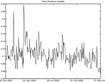
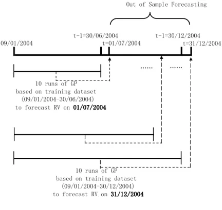
The estimated RV is in Fig. 1. The first six months data is used for initial in-sample training with the out-of-sample testing taking place during the final six months (129 trading days) of the year. Each day’s forecast of RV is determined using all data available up to and including the previous day. For the first day’s out-of-sample forecast (commencing on the first day of July), data from January 9th to June 30th is used. For the last day’s forecast (the last day of December), data from January 9th to December 30th is used. The first five days in January are excluded as lagged information is required in the modelling process.
020.04−Jan−2004 02−Apr−2004 02−Jul−2004 01−Oct−2004 31−Dec−2004 0.06
0.08 0.1 0.12 0.14 0.16 0.18 0.2 0.22 0.24
Fitted Realised Volatility
Fig. 1. Annualised Daily Realised Volatility TABLE I
POTENTIALEXPLANATORYFACTORSUSED INGP
RV Lagged information (one to five days lag) Absolute difference of day open and close price Absolute difference of day highest and lowest price Daily total trading volume
Average five-minute trading volume Daily transaction number
Average daily absolute difference of bid and ask price Maximum daily absolute difference of bid and ask price
Implied volatility(IV) of at money option with one month to expire Average daily trading duration in second
Squared daily return Squared RV
IV lagged information (two to five days lag) Daily Libor
Weekly Libor Six-month Libor
B. GP Approach
In this study we employ GP for symbolic regression. The target variable is realised volatility and the evaluation of an individual GP tree is therefore an RV forecast. The available GP terminal set is outlined in Table I and the available function set is described in Table II. The RV lagged information is the RV on one to five days before the corresponding forecasted day. The average daily trading duration gives the daily averaged information how often a trade happens. The Implied Volatility (IV) is estimated from the FTSE 100 index options data. The factors in Table I are from the previous day’s information if no explicit lag indication given.
Each GP individual has a fitness value which indicates how good they are when tested in-sample on the training dataset. The fitness function in this application is the mean squared error as defined in Eq. 3, where theRVtarget is the
TABLE II
FUNCTIONSETAVAILABLE TOGP
Addition Subtraction Multiplication Division
Cumulative Distribution Function of Normal Distribution Exponential Function
Nature Logarithm Function Square Root
Cube Root Sine Function Cosine Function
target RV value,RVindis the evaluation of the individual and N umberDays is the number of data points in the training
dataset.
F itness=
# $
(RVtarget−RVind)2
N umberDays (3)
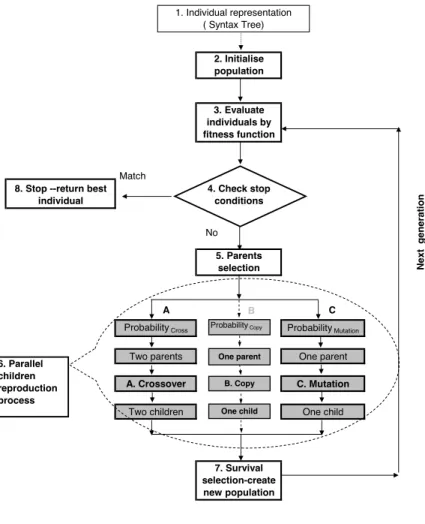
In the experiments, all results are reported averaged across 10 runs and each GP run consists of 50,000 individuals evolved over 50 generations. During each GP run, the new population will be filled by three methods from the old generation. 55 percent of the population will be filled by a crossover method, 40 percent from a mutation method, and 5 percent from reproduction. The GP operation is in Fig.2 The training dataset is used by a method where all available past data is always used. Due to the large computation requirement, only 10 training runs for each forecasted day in the out-of-sample were done in the application. In the future the training tests should be increased. In order to reduce the chance of over-fitting, the maximum tree depth is set to six, based on initial experimentation. The training process is summarized in Fig.3. C. HAR model
In the Heterogeneous Autoregressive model (HAR) [28], RV is modelled by its own lagged information, including RV one day before, average RV in the last week and average RV in the last month. This model is in Eq. 4, where c,α,β andγ are constant coefficients.
RVt=c+αRVt−1+βRVw+γRVm RVw=15$5i=1RVt−i,
RVm= 211 $21i=1RVt−i
(4) The model coefficients are re-trained for each forecasted day. I.e. the training data is used in the same way as discussed in Section III-A.
IV. RESULTS
The out-of-sample results from our experiments are reported in this section. Initially, we report the forecast errors for each modelling methodology, then we present a statistical analysis of these results. Finally, we report the results from a series of information encompassing tests.
A. Forecast Errors
The forecast errors are presented in Table III. In this table, three measures of forecast error (MAE, MAPE and RMSE) are presented for GP and the benchmark approach (HAR). The final column in the table presents theR2 from the linear
regression which regresses the actual RV against the predicted values from each method. The results indicate that using the average of the GP model’s predictions gives the smaller MAE, MAPE and RMSE and also a notably higher correlation in terms ofR2. For each of these error measures, the GP method
reduces the error more than 7% and increasedR2 by 29.3%
when compared with HAR. B. Statistical Analysis
A series of statistical tests were undertaken to determine the significance of the results in Table III. Diebold-Mariano tests including the asymptotic test, sign test and Wilcoxon’s signed test are undertaken on a pair-wise basis for the two competing models on the full out-of-sample time period. The resulting statistics are provided in Table IV. The null hypothesis, that two models give equal results in terms of forecasting accuracy, will be rejected at a 5 percent level if the relevant reported test statistic|X|>1.96.
The results from all three statistical tests give consistent results, that the prediction from GP is significantly different, from that produced by the HAR model, and as already seen in Table III, the GP forecasts produced lower error measures (and higherR2) than the benchmark model. The null hypothesis of
no difference, is rejected by three Diebold-Mariano tests at a 5 percent level.
C. Information Encompassing Tests
These tests are used to determine whether one of a pair of forecasts contains all the useful information for a forecast, or conversely, does a forecast contain additional information not captured by the other. In this case, use of a combination of the forecasts can produce a better forecast than either alone. The forecast information encompassing tests are performed using regression analysis on the full out-of-sample time period and the results are displayed in Table V.
RV =α+βP redicted (5)
Initially, a single factor analysis is performed for each model, where RV is the dependent variable and the prediction from each model is the explanatory variable as in Eq. 5. The results from this are reported in Table V. In evaluating these results it is important to distinguish between bias and predic-tive accuracy. In this single factor analysis, the prediction is unbiased only if α= 0 andβ = 1. The predictive power is indicated byR2. A higherR2means higher predictive power.
Ideally, we seek a forecast with low residual error and highR2
[2]. While it might appear that bias is always undesirable, it should be noted that a biased forecast can still have predictive utility, and conversely an unbiased forecast is of little use if the forecast errors produced by it are large.
2. Initialise population
3. Evaluate individuals by fitness function
4. Check stop conditions
5. Parents selection
Probability Cross Probability Mutation
Two parents One parent
A. Crossover C. Mutation
Two children One child
7. Survival selection-create new population 8. Stop --return best
individual
Match
No
N
e
x
t
g
e
n
e
ra
ti
o
n
Probability Copy
One parent
One child B. Copy
1. Individual representation ( Syntax Tree)
A B C
6.Parallel children reproduction process
Fig. 2. Flow Chart of GP Process TABLE III
OUT-OF-SAMPLEFORECASTERRORMEASURE
Model MAE MAPE RMSE R2
HAR 0.014306 0.158370 0.017351 30.42% GP-avg 0.013060 0.142854 0.016081 39.32% Relative Change -8.71% -9.80% -7.32% 29.26%
TABLE IV
OUT-OF-SAMPLERESULTSSIGNIFICANCETESTS
Diebold-Mariano Tests Test Statistics H0: Equally Accuracy Results
Asymptotic test 3.3858 Rejected at 5%
Sign test 2.5533 Rejected at 5%
Wilcoxon’s signed test 3.4519 Rejected at 5%
The coefficients fitted in the single factor regression analysis in Table V shows that forecast results from HAR are closer to an unbiased prediction than those produced by GP. The intercept αare very close to zero and the coefficient for the model prediction, β are closer to one in HAR model. In the GP case,αis significant as it is not zero at the 5 percent level and the β (1.2813) is significantly higher than one. However, indicated byR2the prediction power from GP is much higher
than the other model and hence it has significant utility despite its bias element.
The second fold of the information encompassing tests is to add the extra prediction results from another model to the right-hand side of Eq. 5 as a second regressor. An increased adjustedR2indicates that the first model can not subsume the
second model and the second model does give extra prediction power. In other words, we are testing whether adding the prediction result from a second model as an extra explanatory factor can further improve the prediction result.
The adjusted R2 is 40.20 percent for the regression when
!"#$%&$'()*+,$-%.,/(0#123
#4567898:9;88< #4567895;9;88< #67595;9;88< ==
#%$&%.,/(0#$>?$%2$!"#!$#%!!&!"#!$#%!!&!"#!$#%!!&!"#!$#%!!&
#68598@9;88<
A(0,B$%2$#.(12123$B(#(0,#$58$."20$%&$CD$ E8F9859;88<47898:9;88<G 8F9859;88<
58$."20$%&$CD$ A(0,B$%2$#.(12123$B(#(0,#$
E8F9859;88<47895;9;88<G #%$&%.,/(0#$>?$%2$'"#"%#%!!&'"#"%#%!!&'"#"%#%!!&'"#"%#%!!&
==
Fig. 3. Overview of GP application for RV Forecasting TABLE V
OUT-OF-SAMPLEFORECASTINFORMATIONENCOMPASSINGTEST
Model α p-Value β p-Value R2 Adj-R2
HAR -0.0048 0.7302 1.0043 0.0000 30.42% 29.87% GP-avg -0.0302 0.0346 1.2813 0.0000 39.32% 38.84%
for RV. An increased adjusted R2 indicates that the second
prediction has extra information, which is not included in the first model. The adjustedR2 of the regression where HAR is
the single explanatory variable for RV is 29.87 percent. When the prediction from GP is added as the second explanatory factor the adjustedR2improves to 40.20 percent. As such, the
prediction of HAR does not subsume the prediction of GP. In contrast, the adjusted R2 from the regression RV against the
prediction from GP is 38.84 percent, which is also lower than 40.20 percent therefore the prediction result from GP does not fully subsumes the prediction from HAR. This suggests that a joint forecast from the GP and HAR model could potentially increase the predictive power.
From the empirical results, GP produces better forecasts than the benchmark model. There are two plausible reasons for this. First, GP takes account of market conditions (as inputs) in forecasting RV. Second, GP permits the use of non-linear functional forms between the RV and market conditions.
It is found from GP returned solutions that some factors including RV with one day and five days lag and average trading duration have occurred frequently. The relationship between these factors and RV seem robust over time. However, their contribution to RV forecasting at different time periods
vary.
V. CONCLUSIONS
Forecasting daily returns volatility is crucial in finance. Tra-ditionally, volatility is modelled using a time-series of lagged information only, an approach which is in essence atheoretical. Although the relationship of market conditions and volatility has been studied for decades, we still lack a clear theoretical framework to allow us to forecast volatility, despite having many plausible explanatory variables. This setting of a data-rich but theory-poor environment suggests a useful role for powerful model induction methodologies such as Genetic Programming. This study forecasts one-day ahead realised volatility (RV) using a GP methodology that incorporates information on market conditions including trading volume, number of transactions, bid-ask spread, average trading dura-tion and implied volatility. The forecasting result from GP is significantly better than that produced by the heterogeneous autoregressive model (HAR), the benchmark model from the traditional finance literature. The error measures and R2
indicate that GP provides a better estimator, and Diebold-Mariano tests confirm that this result is statistically significant. Further, the regression-based Information Encompassing Tests
show that the forecasts from GP contain information not captured by the benchmark model, which indicates that a combination forecast from GP and the conventional model could potentially improve the forecast performance further. In the future, the GP performance can be tested against other conventional models including a hybrid HAR model, which includes all potential factors used in GP as extra explanation variable in RV forecasting.
ACKNOWLEDGMENT
This publication has emanated from research conducted with the financial support of Science Foundation Ireland under Grant Number 08/SRC/FM1389.
REFERENCES
[1] W.K.H. Fung and D.A. Hsieh. “Empirical Analysis of Implied Volatility: Stock, Bonds and Currencies,” presented at the 4th Annu. Conf. of the Financial Operations Research Center, University of Warwick, Coventry, England, 1991.
[2] S.H. Poon and C.W.J. Granger. “Forecasting Volatility in Financial Markets: A Review.”Journal of Economic Literature,vol. XLI, pp. 478-539, 2003.
[3] Koza J.R.,Bennett F.H., Andre D. and Keane, M.A. (1999)Genetic Programming III: Darwinian Invention and Problem Solving, Mor-gan Kaufmann.
[4] Poli R., Landon W.B. and McPhee N.F (2008)A field guide to ge-netic programming, Published viahttp://lulu.comand freely available: http://www.gp-field-guide.org.uk
[5] S.-H. Chen and C.H. Yeh “Using Genetic Programming to Model Volatility in Financial Time Series: the Case of Nikkei 225 and S&P 500.” inProc. of the 4th JAFEE International Conference on Investments and Derivatives(JIC’97), Aoyoma Gakuin University, Tokyo, Japan, July 29-31, 1997, pp.288-306.
[6] R.F. Engle. “The Econometrics of Ultra High Frequency Data.”
Econometrica,vol. 68, pp. 1-22, 2000.
[7] G. Zumbach, O.V. Pictet and O. Masutti. (2001, Apr.)“Genetic Pro-gramming with Syntactic Restrictions Applied to Financial Volatility Forecasting.” Olsen & Associates Working Paper. [online] Paper No. GOZ.2000-07-28. Available: http://ssrn.com/abstract=269189[15 Dec. 2006].
[8] C.J. Neely and P.A. Weller “Predicting Exchange Rate Volatility: Genetic Programming Versus GARCH and RiskMetricsT M.” The Federal Reserve Bank of St. Louis, May/June, 2002.
[9] I. Ma, T. Wong , T. Sankar and R. Siu “Forecasting the Volatility of a Financial Index by Wavelet Transform and Evolutionary Algorithm.” inProc. of the 2004 IEEE International Conference on Systems, Man and Cybernetics, 2004, pp.5824-5829.
[10] S. B. HAMIDA and R. Cont. “Recovering Volatility from Option Prices by Evolutionary Optimization.” Journal of Computational Finance, vol. 8, No. 4, Summer 2005.
[11] W. Abdelmalek, S. B. Hamida and F. Abid. (2009). “Select-ing the Best Forecast“Select-ing-Implied Volatility Model Us“Select-ing Ge-netic Programming.” Journal of Applied Mathematics and Deci-sion Sciences.[online]. vol. 2009, Article ID 179230. Available: http://www.hindawi.com/journals/ads/2009/179230/ [17 Sep.2011]. [12] H.M. Wu and W.C. Guo. “Asset Price Volatility and Trading Volume
with Rational Beliefs.”Economic Theory, vol. 23, no. 4, pp. 795-829, Jun. 2004.
[13] H.C. Chena and J. Wu. “Return Volatility and the Intraday Behavior of Market Liquidity without Market Makers: Evidence from the Taiwan Futures Market.”International Research Journal of Finance and Economics,issue 17, pp. 117-128, Jul. 2008.
[14] S.J. Taylor. “Forecasting the Volatility of Currency Exchange Rates.”
International Journal of Forecasting,vol. 3, pp. 159-170, 1987. [15] L.R. Glosten, R. Jagannathan and D.E. Runkle. “On the Relation
between the Expected Value and the Volatility of the Nominal Excess Return on Stocks.”The Journal of Finance,vol. 48, no. 5, pp. 1779-1801, 1993.
[16] M. Ammann, D. Skovmand and M. Verhofen. “Implied and Realized Volatility in the Cross-Section of Equity Options.” International Journal of Theoretical and Applied Finance, vol. 12, issue 6, pp. 745-765, 2009.
[17] G.H.K. Wang and J. Yau. “Trading Volume, Bid-Ask Spread, and Price Volatility in Futures Markets.” Journal of Futures Markets,
vol. 20, issue 10, pp. 943-970, 2000.
[18] M. McAleer and M.C. Medeiros. “Realized Volatility: A Review.”
Econometric Reviews,vol. 27(1-3), pp. 10-45, 2008.
[19] T.G. Andersen, T. Bollerslev, F.X. Diebold and P. Labys. “Modeling and Forecasting Realized Volatility.”Econometrica,vol. 71, pp. 529-626, 2003.
[20] T.G. Andersen and T. Bollerslev. “Answering the Skeptics: Yes, Stan-dard Volatility Models Do Provide Accurate Forecasts.”International Economic Review,vol. 39, no. 4, pp. 885-905, 1998.
[21] N.M.P.C. Areal and S.J. Taylor. “The Realized Volatility of FTSE 100 Futures Prices.”Journal of Futures Markets,vol. 22, issue 7, pp. 627-648, 2000.
[22] D.D. Thomakos and T. Wang. “Realized Volatility in the Futures Markets.”Journal of Empirical Finance,vol. 10, pp. 321-353, 2003. [23] F. Corsi “A Simple Long Memory Model of Realized Volatility.”
Working Paper, University of Southern Switzerland, vol. 71, pp.529-626, 2003.
[24] Y. A¨ıt-Sahalia and L. Mancini. “Out of Sample Forecasts of Quadratic Variation.”Journal of Econometrics,vol. 147, pp. 17-33, 2008.
[25] L. Xiao. “Realized Volatility Forecasting: Empirical Evidence from Stock Market Indices and Exchange Rates.”Applied Financial Eco-nomics,vol. 23, pp. 57-69, 2013.
[26] F. Corsi, S. Miittnik, Ch. Pigorsch and U. Pigorsch. “The Volatility of Realized Volatility.”Econometric Reviews,vol. 27, pp. 46-78, 2008. [27] T.G. Andersen, T. Bollerslev and F.X. Diebold. “Roughing It Up: Including Jump Components in the Measurement, Modeling and Forecasting of Return Volatility.”Review of Econometrics and Statis-tics,vol. 89, pp. 701-720, 2007.
[28] F. Corsi. “A Simple Approximate Long-Memory Model of Realized Volatility.”Journal of Financial Econometrics,vol. 7, no. 2, pp. 174-196, 2009.
[29] A.M. Fuertes, M. Izzeldin and E. Kalotychou. “On Forecasting Daily Stock Volatility: The Role of Intraday Information and Market Conditions.”International Journal of Forecasting,vol. 25, pp. 259-281, 2009.
[30] N.K. L´eon. (2008)“The Effects of Interest Rates Volatility on Stock Returns and Volatility: Evidence from Korea.”International Research Journal of Finance and Economics.[online]. ISSN 1450-2887, is-sue 14. Available: http://www.eurojournals.com/finance.htm[1 Jan. 2012].
[31] N. Zafar, S.F. Urooj and T.K. Durrani. (2008) “Interest Rate Volatility and Stock Return and Volatility.”European Journal of Economics, Finance and Administrative Sciences.[online]. ISSN 1450-2887, is-sue 14. Available: http://www.eurojournals.com[1 Jan. 2012]. [32] S. Rahman, C.F. Lee and K.P. Ang. “Intraday Return Volatility
Process: Evidence from NASDAQ Stocks.”Review of Quantitative Finance and Accounting,vol. 19, pp. 155-180, 2002.
[33] E. Kalotychou and S.K. Staikouras. “Volatility and Trading Activity in Short Sterling Futures.” Applied Economics, vol.38, no. 9, pp. 997-1005, 2006.
[34] C.M. Jones and G. Kaul. “Transactions, Volume, and Volatility.”The Review of Financial Studies,vol. 7, no. 4, pp. 631-651, 1994. [35] L.R. Glosten, R. Jagannathan and D.E. Runkle. “On the Relation
between the Expected Value and the Volatility of the Nominal Excess Return on Stocks.”The Journal of Finance,vol. 48, no. 5, pp. 1779-1801, 1993.
[36] A.F. Darrat, S. Rahman and M. Zhong. “Intraday Trading Volume and Return Volatility of the DJIA Stocks: A Note.” Journal of Banking & Finance,vol. 27, pp. 2035-2043, 2003.
[37] C. Brooks. “Predicting Stock Index Volatility: Can Market Volume Help?”Journal of Forecasting,vol. 17, pp. 59-80, 1998.