ASTRONOMY
AND
ASTROPHYSICS
Disturbing function in the analytical theory of the motion of Phobos
Piotr Wa¸˙z
Centrum Astronomii, Uniwersytet Mikol´aja Kopernika, ul. Gagarina 11, PL-87-100 Toru´n, Poland Received 27 November 1999 / Accepted 12 May 1999
Abstract. A new theory of the motion of Phobos – the moon
of Mars – is created. The accuracy of this theory is to within one meter of the mean motion of Phobos over one year which is the best result obtained so far for the analytical approach. The perturbational analysis is of main interest. The elements of the physical interactions which are the most essential for the motion of Phobos are specified. The theory is based on the two fixed gravitational centers problem. Analytical functions of this problem are expressed as a series of the third order with respect to the J2 and J3/J2 zonal harmonics of Mars. This theory takes into account the interaction of Phobos with the potential of Mars consisting of very many elements. The zonal harmonics of order≤12and tesseral harmonics of order≤6 are considered. Interactions of Phobos with the Sun, Jupiter, Deimos – another moon of Mars, and the tidal potential of the Sun are taken into account. The influence of all the elements of the perturbational function on the accuracy for determining the position of Phobos is presented. The numerical integration allows to illustrate the influence of all perturbations (of the ones which have been taken into account and of the ones which have been neglected) on the mean motion of Phobos.
Key words: planets and satellites: individual: Phobos – celestial
mechanics, stellar dynamics – methods: analytical
1. Introduction
The aim of this paper is the creation of an analytical theory of the motion of Phobos, which would be accurate enough to analyse currently available observational data and that expected from future observations.
The theory developed in this paper has been derived from the model of the two fixed gravitational centers (Aksenov 1977, Emelianov et al., 1984, 1993). The results are aimed at estab-lishing links between the observed perturbations and the real physical factors which are responsible for these perturbations.
The pilot results presented in this work show, that the ex-isting theories, even the most accurate ones, do not take into account all the forces acting on Phobos up to the assumed pre-cision (Born et al., 1975, Chapront-Touz´e, M. 1988, Emelianov
Send offprint requests to: Piotr Wa¸˙z
et al., 1984, 1993, Jacobson et al., 1989, Morley 1990, Sinclair 1972, 1989, Shor 1975, 1988).
The creation of a good analytical model will not only make possible a reduction in the computations necessary to correct the orbits of the Martian satellites, but may also be used as a starting point for a precise description of other objects, as e.g. the artificial satellites of Mars which will be launched in the future.
During the next two decades several missions to the area of Mars are planned. Their main goal is a preparation for the landing of man on Mars. A precise knowledge of the phenomena which may influence the motion of all objects in the proximity of Mars is a prerequisite for the success of this project.
The formulation of the equations of motion is the most im-portant step in creating a theory of the motion. Apart from the problems relating to the choice of the system of the coordinates, to the choice of the variables and to the expansion of the per-turbational function, the most important is the decision as to which physical interactions in the system under consideration are nonnegligible.
The aim of this paper is to analyze the motion of Phobos us-ing a theory which, as accurately as it is possible, would describe the influence of the gravitational interactions so as to facilitate the derivation of any hypothetical perturbations of another ori-gin from the observational data. An analysis of the gravitational forces acting on Phobos and the way of the expansion of the perturbational function are presented in this paper.
The Hamiltonian formalism is used for the mathematical de-scription of the problem. The Hamilton functions of the problem may be written as:
K=K0+Kp, (1)
whereK0 is the Hamiltonian of the problem of the two fixed gravitational centers andKp contains the terms describing all the other interactions which are taken into account.
The perturbational function consists of the zonal harmonics of the order not larger than 12 and of the tesseral harmonics of the order not larger than 6, except for the harmonics in which the first index is equal to 6 and the second one is odd. The inter-actions with the Sun, with Deimos and with Jupiter as well as the tidal potential of the Sun are taken into account. The inertial forces, resulting from the choice of the non-inertial coordinate
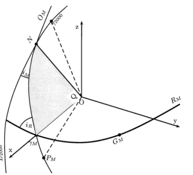
Fig. 1. Reference frame.
system are also introduced. The perturbational function is at most of the second order with respect to the small parameters of the intermediate orbit. The basic problem is written up to the third order. Therefore all the parameters of the perturbational function which describe the intermediate orbit have to be ex-pressed up to the first order. All interactions smaller than the truncated part ofK0are neglected. Before analyzing the per-turbational function, let us choose the variables in which the Hamilton function will be expressed. This choice is determined by two basic factors. First they must be appropriate for the de-scription of the intermediate orbit described byK0. Secondly, these variables should be useful for the next level of the theory, i.e. for the analytical integration of the equations of the motion. These conditions are fulfiled by the variablesa,e,s,l,g andh. As in the case of the Kepler orbit,astands for the semi-major axis, e – for the eccentricity, s – for the sine of the angle of inclination of the orbit to the reference plane, the anglesl, gandh(up toJ2andJ3/J2) are the counterparts of the mean anomaly, the argument of the pericentre and the longitude of the node of the satelite orbit.
The power series expansion of the Hamiltonian is performed using the PSPC program developed by Dr. Alberto Abad and Juan Felix San-Juan 1994 from the University of Zaragoza.
The form of the perturbational function depends on the choice of the reference frame. Fig. 1 presents the chosen ref-erence frame. The origin of the coordinates is the center of gravity of Mars. The 0xy plane is the Martian mean equator of dateRM, the x axis pointing towardsγM, the ascending node ofRM on Mars mean orbit of dateOM.E2000is the mean dy-namical ecliptic andγ2000is equinox ofJ2000. The inclination ofOM onE2000is denoted asiMand the inclination ofRMon OMis denoted asiR.Qstands for the arcNγM.GMstands for
the intersection of the prime meridian of Mars withRM.
Fig. 2. ilustration of the problem
2. Two fixed gravitational centers
The problem of the two fixed gravitational centers has been formulated and solved by Leonard Euler. The aim of his study was to find the motion of a material pointm0in a potential U =f m1 r1 + m2 r2
defined as a sum of two Newton potentials generated by two material points m1 andm2 located in two fixed positions in the Oz axis of a coordinate systemOxyz.f is the universal gravitational constant. The distances fromm1andm2tom0,r1 andr2respectively, may be expressed by the distances from the origin of the coordinate system tomand by two constants,c1 andc2, describing the positions ofm1andm2on theOzaxis. After some algebra one obtains
UE=f(m1r+m2) " 1−X∞ k=1 γ0 k rkPk z r # , (2) where (m1+m2)γ0k=m1ck1+m2ck2.
The gravitational potential of an arbitrary body in the Solar system is rather complicated. In particular it is not spherically symmetric, as it would be in the case of the Newton potential. Assuming a cylindrical symmetry of the potential relative to the polar axis, the potential may be written as:
UN = f(rm) " 1− ∞ X k=2 Jkr k 0 rkPk z r # , (3)
wherer0is the equatorial radius of the central mass,mis the mass of the body andzis the coordinate of them0.
Before comparing Eqs. (3) and (2) let us introduce parameter r0to Eq. (2). Then UE=f(m1r+m2) " 1− ∞ X k=1 γkr k 0 rkPk z r # . (4)
Expansion (4) contains four independent parameters:m1,m2, c1andc2. Therefore only four terms in expansion (3) may be identified with appropriate terms in expansion (4). If this is done for the first four terms of the expansion, one obtains: m = m1 +m2, γ2 = J2 andγ3 = J3. The remaining terms in these expansions are not equal. Only several initialγkvalues are known with an adequate accuracy. The values of the remaining ones are not known very well, however they are very small. As a consequence, the approximation (3) to the potential (4) is usually good.
The value ofJkhas been taken from Smith et al 1993. The values ofγkhave been obtained from the theory of the two fixed gravitational centers (see Aksenov 1977).
k Jk γk 2 1.9587441×10⁻³ 1.9587441×10⁻³ 3 3.1500844×10⁻⁵ 3.1500844×10⁻⁵ 4 -1.5447300×10⁻⁵ -3.3300768×10⁻⁶ 5 5.8488678×10⁻⁶ -1.1525693×10⁻⁷ 6 -4.8098054×10⁻⁶ 4.6691875×10⁻⁹ 7 -5.0445608×10⁻⁶ 3.0084948×10⁻¹⁰ 8 -4.4323385×10⁻⁷ -4.3074328×10⁻¹² 9 8.3865216×10⁻⁷ -6.5855998×10⁻¹³ 10 -3.2527122×10⁻⁶ -2.1539114×10⁻¹⁵ 11 1.9490259×10⁻⁶ 1.2553110×10⁻¹⁵ 12 -5.1900000×10⁻⁷ 2.4407078×10⁻¹⁷
The solution of the problem of the two fixed gravitational centers is very complicated. Whenever it is required by the clarity of the presentation, formulae which appear in the problem of the two fixed gravitational centers are customarily expressed as series of small parameters: ε2= c2 a2(1−e2)2 and εσ = cσ a(1−e2), where c=r0 s J2− J3 2J2 2 , σ= J3 2J2 r J2− J3 2J2 2.
These constants are linked to the problem of the two fixed cen-ters by:
m1= m2 (1 +iσ) , m2=m2 (1−iσ) , c1=c(σ+i) , c1=c(σ−i) , wherei=√−1.
The Hamiltonian describing the motion of a body in the potential (2) expressed in terms of the elementsa,e,s,Ω0,ω0 andM0, which have been used to describe the Eulerian orbit, reads:
K0 = fm2a 1−ε2(1−s2)(1−e2) + ε4s2(1−s2)(1−e2)(3 +e2) + ε4σ2(1−s2)(1−e2)(−1 + 7s2)−
ε6s4(1−s2)(1−e2)(5 + 10e2+e4)+· · ·,
where the elements up the third order with respect to ε2 and εσhave been written explicitly.fis the universal gravitational constant andmis the sum of the masses of Mars and Phobos. Under the assumption ofc= 0andσ= 0, the elementsa,e,s,
Ω0,ω0 andM0 become equal to the corresponding Keplerian elements: i.e. the semi-major axis, the eccentricity, the sine of the inclination of the orbit to the reference plane, the longitude of the node, the argument of the pericentre and the mean anomaly, respectively. This way of expressingK0is not very convenient for the process of the analytical integration. The equations of the perturbational motion may be, most conveniently, expressed in terms of the elementsL,G,H,l,gandh(Aksenov 1977), which forc = 0andσ = 0become equal to the elements of Delaunay.
3. The main problem
The main part of the Hamilton function expressed in terms of the “Delaunay variables” reads:
K0 = (fm) 2 2L2 − c2(fm)4 4G5L3 (G2−3H2)− (5) c2σ2(fm)4 4G5L3 (G2−3H2)− 3c4(fm)6 64G11L5(2G6− 36G4H2+ 50G2H4−2G5L+ 12G3H2L− 18GH4L−5G4L2+ 70G2H2L2−105H4L2)− 3c4σ2(fm)6 32G11L5 (G6−18G4H2+ 25G2H4− 2G5L+ 12G3H2L−18GH4L−2G4L2+ 16G2H2L2−30H4L2)− c6(fm)8 256G17L9(12G10L2−462G8H2L2+ 1920G6H4L2−1710G4H6L2−30G9L3+ 630G7H2L3−2370G5H4L3+ 2250G3H6L3− 62G8L4+ 3658G6H2L4−11754G4H4L4+ 11334G2H6L4−765G5H2L5+ 105G6L6+ 2835G3H4L5−2835GH6L5−3465G4H2L6+ 15015G2H4L6−15015H6L6+ 45G7L5)· · · The limitation of the theory to the third order is a necessary com-promise between an attempt to create a very accurate analytical theory (leading to a very large expansion of the perturbational function) and the practical limitations imposed by the afford-able computational time. In order to estimate the value ofK0 let us take the well known Kepler equation:
K0≈n 2a2 2 , (6) where n= r fm a3 .
The error in this estimation is determined by the values of the small parameters (ε2,εσ) of the problem of the two fixed grav-itational centers. It is estimated to be about10−3. The set of values needed for this estimation is:
– n= 1128.84426◦d−1– the mean motion of Phobos,
– fm= 42828.28km3s−2 – a= 9373.71565km.
The following system of units is used in this work:
– time - 24 hours =d,
– length - the equatorial radius of Mars,r0= 3394.2km. Using these values one obtains K0 ≈ 1.5×10³r20/d2. For e= 0.015,s= 0.018and for the values listed above the value of the third-order terms inK0
∆K0=ε6n 2a2 2 ≈2×10⁻⁸ r2 0 d2. (7)
All the contributions of the perturbational function which are equal or greater than∆K0are taken into account in this theory. If the perturbational function is determined with this accuracy and the constants are taken from (6) then the order of the error of the resulting secular effects in the motion of Phobos is 1 meter/year.
Expressing the perturbational function in terms ofL,G,H, l,g,h, is very cumbersome. Therefore another set of elements in order to expressK0 in a simpler way has to be introduced. The new set of elements (a,e,s,l,g,h) is a composition of the elements of the intermediate orbit with the original elementsL, G,H,l,g,h. The elementsa,e,s,l,g,hforc= 0andσ= 0 are equivalent to the osculation elements of the Kepler problem.
4. Disturbing function – Mars potential
The perturbational function describing the influence of pertur-bations due to non-uniformity of the gravitational potential of Mars (denoted byh) is:
Kh p =fm ∞ X n=2 n X k=0 jn kRe{Rn k} , (8) where Rn k= r n 0 rn+1Pn k(sinϕ) exp √ −1k(λ−wnk). (9) ϕandλare respectively the latitude and longitude of Phobos in the defined coordinate system,wnk,jn k are the constants describing the nonspherical potential of Mars,Re{Rn k}is the real part ofRn k,Pn kare the associated Legendre polynomials andris the radius of the orbit of Phobos. Let us replaceλin the above equation byα−Gt,whereαmeans right ascension andGtis the sidereal time defined for Mars. The Eq. (9), after multiplying byexp√−1(ˆΩ−ˆΩ)reads:
Rn k = r n 0 rn+1Pn k(sinϕ) exp √ −1k(α−ˆΩ) exp√−1kˆΩ exp√−1k(−Gt−wnk),
where ˆΩis the longitude of the node determined up to the ac-curacy of the small parameter.
The part of the perturbational function which depends only on the zonal harmonics (8) (denoted byzh) may be identified by taking thek= 0terms in the corresponding expansion: Kzh p =fm ∞ X n=4 jn r n 0 rn+1Pn(sinϕ) = ∞ X n=4 Kzh p n, (10)
wherejn ≡jn0,Pn ≡Pn0. In order to estimate the terms of this series for the model of the 50th I use the results given in paper Smith et al., 1993. Let us assume that the orbit of Phobos is circular and the angle between its plane and the reference plane is equal to sinϕ = 0.02. The major terms of the Pn(sinϕ) corresponding to even values ofnmay be approximated by
(−1)n2 n!
2n(n
2!)2
and the ones corresponding to oddnby
(−1)n−21 (n−1)!
2n(n−1 2 !)2
sinϕ.
In particular the major terms of theKpnzhfunction are the fol-lowing: Kzh p4≈2×10⁻⁴r20/d2, Kpzh5≈ −4×10⁻⁶r20/d2, Kzh p6≈ −1×10⁻⁵r02/d2, Kpzh7≈ −5×10⁻⁷r20/d2, Kzh p8≈ −1×10⁻⁷r02/d2, Kpzh9≈ −1×10⁻⁸r20/d2, Kzh p10≈ −9×10⁻⁸r02/d2, Kpzh11≈4×10⁻⁹r02/d2, Kzh p12≈2×10⁻⁹r20/d2 and n jn=−(Jn−γn) 2 0 3 0 4 1.2117223×10⁻⁵ 5 -5.9641248×10⁻⁶ 6 4.8144746×10⁻⁶ 7 5.0448617×10⁻⁶ 8 4.4322957×10⁻⁷ 9 -8.3865281×10⁻⁷ 10 3.2527122×10⁻⁶ 11 -1.9490259×10⁻⁶ 12 5.1900000×10⁻⁷
The above terms are greater than∆K0defined by the Eq. (7) so they are taken into account as a contribution to the perturbational function.Kpzh9,Kpzh11andKpzh12do not fulfil the condition of preassumed accuracy. However these three terms are taken into account as a contribution to the perturbational function because in this way the sum of all the rejected terms is smaller than
∆K0. All the other terms smaller than∆K0are not taken into account and have not been written.
Let us express the functionKpzhin terms ofa, e, s, l, g, and h. The basic Hamiltonian has been expanded in terms of the small parameters up to the third order. All terms in the pertur-bational potential are of at most second order. Therefore the relations between the elements of the intermediate orbit should
be given up to the first order. Using the results of Emelianov et al., 1984 one obtains:
sinϕ = ssinθ 1−2cξ22(1−s2sin2θ)− (11) c ξ+ ε σssinθ +cσξ −εσ(1−2s2).
εis the parameter connected to the problem of the two fixed gravitational centers and
ξ = ξ0
1 +ε24s2e(1 +ecosφ) sinφsin(2φ+ 2g)− (12) ε2e2(1−s2) sin2φ, where ξ0= a(1−e 2) 1 +ecosφ, (13) θ = u+ν(φ−l)−ε2s2esinφ− (14) 1 2ε2e2 1 −34s2sin 2φ+ ε2s2
8 sin(2φ+ 2g)(3 + 4ecosφ+e2cos 2φ).
u=φ+g, whereφis a true anomaly of the orbit of Phobos. The difference betweenθanduis of the order of a small parameter. Therefore one can write:
exp√−1(n−2l)θ= (1 + ∆u) exp√−1(n−2l)u, (15) ∆u = √−1(n−2l) h ν(φ−l)−ε2es2sinφ− (16) 1 2ε2e2 1−34s2sin 2φ +18ε2s2(1−e2) sin 2u+ ε2s2 4 sin 2u(1 +ecosφ)2 , where ν =34ε2(4–5s2) (17) and φ−l= 2p1−e2 ∞ X p=1 χ−2,0 p (e)sinppl. (18)
χ
are the coefficients of Hansen. In order to obtain the expansion of1/rn+1let us expressras:r=ξ0(1 + ∆r), (19) where ∆r = εσs(1−e2)ξa 0sinu+ 1 4ε2(1−e2)2 (20) (2−s2)a ξ0 2 +14ε2(1−e2)2s2a ξ0 2 cos 2u− ε2e2(1−s2) sin2φ+ 1 4ε2s2e(1−e2) a ξ0sinφsin 2u. Then 1 rn+1 = 1 ξn0+1[1−(n+ 1)∆r]. (21) The terms containing∆2rand higher powers are neglected (∆r is of the order of the small parameter of the intermediate orbit). Expanding the part of the function corresponding toj4up to the seventh order usingeandsvariables one obtains
j4- 158 terms of the following type: C ε2εσ ν eke sks a−5
sin
cos
(kll+kgg), whereks= 0, ...,5,ke= 0, ...,7, kl= 0, ...,7, kg=−2, ...,5.
In the other cases the series are restricted up to the fifth order usingeands. The result is the following:
j5- the series containing 53 terms C ε2 εσ ν eke sks a−6
sin
cos
(kl l +kg g), where ks = 0, ...,3,5, ke= 0, ...,4, kl= 0, ...,5, kg=−1, ...,3,5, j6- 57 terms, C ε2εσ ν eke sks a−7sin
cos
(kll+kgg), whereks= 0, ...,4, ke= 0, ...,5, kl= 0, ...,5, kg=−2, ...,4, j7- 53 terms, C ε2 εσ ν eke sks a−8sin
cos
(kl l +kg g), where ks = 0, ...,3,5, ke= 0, ...,4, kl= 0, ...,5, kg=−1, ...,3,5, j8- 57 terms, C ε2εσ ν eke sks a−9sin
cos
(kll+kgg), whereks= 0, ...,4, ke= 0, ...,5, kl= 0, ...,5, kg=−2, ...,4, j9- 53 terms, C ε2 εσ ν eke sks a−10sin
cos
(kl l +kg g), whereks = 0, ...,3,5, ke= 0, ...,4, kl= 0, ...,5, kg=−1, ...,3,5, j10- 57 terms, C ε2εσ ν eke sks a−11sin
cos
(kll+kgg), whereks= 0, ...,4, ke= 0, ...,5, kl= 0, ...,5, kg=−2, ...,4, j11- 53 terms, C ε2 εσ ν eke sks a−12sin
cos
(kl l +kg g), whereks = 0, ...,3,5, ke= 0, ...,4, kl= 0, ...,5, kg=−1, ...,3,5andj12- 57 terms,C ε2εσ ν eke sks a−13
sin
cos
(kll+kgg),where ks = 0, ...,4 , ke = 0, ...,5 , kl = 0, ...,5 , kg =
−2, ...,4.
The series corresponding to harmonics with odd indices con-tain secular terms of orderεσ.
The disturbing function for perturbation on the satellite Pho-bos due to the tesseral gravitational field of Mars (denoted by th) is given by: Kth p = fm ∞ X n=2 n X k=1 jn k r n 0 rn+1Pn k(sinϕ)Re{ (22) exp√−1k(α−ˆΩ) exp√−1kˆΩ exp√−1k(−Gt−wnk) = ∞ X n=2 n X k=1 Kth p nk.
In particular the major terms of theKp nkth function are the fol-lowing:
Kth p22≈5×10⁻⁵r02/d2, Kpth51≈ −4×10⁻⁸r20/d2, Kth p31≈4×10⁻⁶r02/d2, Kpth52≈ −2×10⁻⁸r20/d2, Kth p32≈2×10⁻⁷r02/d2, Kpth53≈7×10⁻⁸r20/d2, Kth p33≈ −9×10⁻⁶r02/d2, Kpth54≈1×10⁻⁸r20/d2, Kth p41≈6×10⁻⁸r02/d2, Kpth55≈ −2×10⁻⁷r20/d2, Kth p42≈ −5×10⁻⁷r02/d2, Kpth62≈1×10⁻⁸r20/d2, Kth p43≈ −4×10⁻⁸r02/d2, Kpth64≈ −2×10⁻⁸r20/d2, Kth p44≈1×10⁻⁶r02/d2, Kpth66≈3×10⁻⁸r20/d2 and n,k jnk wnk 2,2 6.3173653×10⁻⁵ 1.3082474 3,1 2.7617341×10⁻⁵ 1.4237084 3,2 6.1543999×10⁻⁶ 1.3309354 3,3 6.0579601×10⁻⁶ 0.20962663 4,1 5.3593895×10⁻⁶ 0.71622562 4,2 2.0212556×10⁻⁶ 2.2977274 4,3 3.8704524×10⁻⁷ 2.0855004 4,4 2.7169253×10⁻⁷ 1.1838778 5,1 1.8214941×10⁻⁶ 1.2779661 5,2 7.0829951×10⁻⁷ 1.7298508 5,3 1.1148785×10⁻⁷ 0.031127582 5,4 4.5006606×10⁻⁸ 0.94805971 5,5 1.4319927×10⁻⁸ 0.48924539 6,2 2.3133193×10⁻⁷ 0.55573885 6,4 1.0807266×10⁻⁸ 0.30838450 6,6 6.8065260×10⁻¹⁰ 0.050312693
The above terms fulfil the condition of preassumed accuracy and all the other rejected terms have not been written. For deriving the functionKpth the expressions (11)-(21) and Emelianov et al., 1984: exp√−1kˆΩ = (1 + ∆Ω) exp√−1kh, (23) where ∆Ω = √−1k µ(φ−l)−32ε2ecosisinφ− (24) ε2e
2 cosisinφ(1 +ecosφ) , µ=ε21 + 1 2e2 p 1−s2
are needed. Writing (Aksenov 1977, Emelianov et al., 1984): Rn k= 2 a r n+1(n−k)! (n+k)!Pn k(sinδ) one obtains: Rn k = ar 2n−1 n+k sinϕRn−1k− n−k−1 n+k a r Rn−2k , Rn k = p2(k+ 1) 1−sin2ϕsinϕRn k+1− (n−k−1)(n+k+ 2)Rn k+2, Rn−1n= 0, Rn n= q 1−sin2ϕn(2n−1)!! , where (2n−1)!! = 1·3·5· · ·(2n−1).
Using the same level of truncation as in the case of the sec-ond group of zonal harmonics and multiplying every term of the series by the corresponding expressionfmjnkrn0/an+1one obtains
j2,2 - 102 terms of the following type: C ε2 εσ ν µ a−3 eke sks
sin
cos
(kl l+kg g+kh h+kG Gt+kww2,2) , whereks = 0, ..,3 , ke = 0, ...,5 ,
kl= 0, ...,5, kg=−2, ...,3, kh=kG=kw= (±2),
j3,1 - 190 terms of the following type: C ε2εσ ν µ a−4ekesks
sin
cos
(kll+kg g+khh+kGGt+kww3,1),whereks= 0, ..,3, ke= 0, ...,5, kl= 0, ...,8,
kg=−3,−1, ...,5, kh=kG=kw= (±1),
j3,2 - 108 terms of the following type: C ε2εσ ν µ a−4eke sks
sin
cos
(kll+kgg+khh+kGGt+kww3,2),whereks= 0, ..,3, ke= 0, ...,4, kl= 0, ...,5, kg=−1, ...,3, kh=kG=kw= (±2),
j3,3 - 136 terms of the following type: C ε2 εσ ν µ a−4 eke sks
sin
cos
(kl l+kg g+kh h+kG Gt+kww3,3) , whereks = 0, ..,3 , ke = 0, ...,4 , kl= 0, ...,5, kg=−2, ...,3, kh=kG=kw= (±3), j4,1 - 119 terms of the following type:
C ε2 εσ ν µ a−5 eke sks
sin
cos
(kl l+kg g+kh h+kG Gt+kww4,1) , whereks = 0, ..,4 , ke = 0, ...,5 , kl= 0, ...,5, kg=−2, ...,3, kh=kG=kw= (±1), j4,2 - 237 terms of the following type:
C ε2 εσ ν µ a−5 eke sks
sin
cos
(kl l+kg g+kh h+kG Gt+kww4,2) , whereks = 0, ..,4 , ke = 0, ...,5 ,
kl= 0, ...,7, kg=−2, ...,4, kh=kG=kw= (±2),
j4,3 - 119 terms of the following type: C ε2 εσ ν µ a−5 eke sks
sin
cos
(kl l+kg g+kh h+kG Gt+kww4,3) , whereks = 0, ..,4 , ke = 0, ...,5 ,
kl= 0, ...,5, kg=−2, ...,3, kh=kG=kw= (±3),
j4,4 - 195 terms of the following type: C ε2 εσ ν µ a−5 eke sks
sin
cos
(kl l+kg g+kh h+kG Gt+kww4,4) , whereks = 0, ..,4 , ke = 0, ...,5 ,
kl= 0, ...,7, kg=−2, ...,4, kh=kG=kw= (±4),
j5,1 - 112 terms of the following type: C ε2 εσ ν µ a−6 eke sks
sin
cos
(kl l+kg g+kh h+kG Gt+kww5,1) ,whereks = 0, ..,3,5, ke= 0, ...,4, kl= 0, ...,5, kg=−1, ...,3,5, kh=kG=kw= (±1),
j5,2 - 112 terms of the following type: C ε2 εσ ν µ a−6 eke sks
sin
cos
(kl l +kg g+kh h+kG Gt+kww5,2),whereks= 0, ..,3,5 , ke= 0, ...,4 , kl= 0, ...,5, kg=−1, ...,3,5, kh=kG=kw= (±2), j5,3 - 112 terms of the following type:
C ε2 εσ ν µ a−6 eke sks
sin
cos
(kl l +kg g+kh h+kG Gt+kww5,3),whereks= 0, ..,3,5 , ke= 0, ...,4 ,
kl= 0, ...,5, kg=−1, ...,3,5, kh=kG=kw= (±3),
j5,4 - 112 terms of the following type: C ε2 εσ ν µ a−6 eke sks
sin
cos
(kl l +kg g+kh h+kG Gt+kww5,4),whereks= 0, ..,3,5 , ke= 0, ...,4 ,
kl= 0, ...,5, kg=−1, ...,3,5, kh=kG=kw= (±4),
j5,5 - 112 terms of the following type: C ε2 εσ ν µ a−6 eke sks
sin
cos
(kl l +kg g+kh h+kG Gt+kww5,5),whereks= 0, ..,3,5 , ke= 0, ...,4 ,
kl= 0, ...,5, kg=−1, ...,3,5, kh=kG=kw= (±5),
j6,2 - 119 terms of the following type: C ε2 εσ ν µ a−7 eke sks
sin
cos
(kl l +kg g+kh h+kG Gt+kww6,2) ,whereks = 0, ..,4 , ke = 0, ...,5 , kl= 0, ...,5, kg=−2, ...,3, kh=kG=kw= (±2), j6,4 - 119 terms of the following type:
C ε2 εσ ν µ a−7 eke sks
sin
cos
(kl l +kg g+kh h+kG Gt+kww6,4) ,whereks = 0, ..,4 , ke = 0, ...,5 , kl= 0, ...,5, kg=−2, ...,3, kh=kG=kw= (±4), j6,6 - 119 terms of the following type:
C ε2 εσ ν µ a−7 eke sks
sin
cos
(kl l +kg g+kh h+kG Gt+kww6,6) ,whereks = 0, ..,4 , ke = 0, ...,5 , kl= 0, ...,5, kg=−2, ...,3, kh=kG=kw= (±6).
5. Disturbing functions – Sun, Deimos, Jupiter
The perturbational function for the Sun (denoted byS) may be written as KS p =fMS ∞ X n=2 rn rn+1 S Pn(cosS), (25) cosS= xxS+rryyS+zzS S . (26)
MS, rSare the mass and the radius of the orbit of the Sun respec-tively,x, y, zare the coordinates of Phobos,xS, yS, zS are the coordinates of the Sun. From a knowledge of the mean motion and the semi-major axis of the orbit of Mars one can estimate the numerical value ofKpS ≈n2Sa2/2≈3.2×10−4r02/d2, where nSis the mean motion of the Sun. Therefore this function may
be taken into account and classified as the second-order one. The form of the perturbational function is already known. The next step is expressing this function in terms of the elements a, e, s, l, g, hof the intermediate orbit and of the timet. Using the formulae from Emelianov et al., 1984 one obtains:
cosϕsin(α−ˆΩ) = p1−s2sinθ 1 + s22ξc22sin2θ− c ξ+ε σssinθ + 2εσsp1−s2,
cosϕcos(α−ˆΩ) = cosθ
1 + 2cξ22s2sin2θ− c ξ+ε σssinθ .
The above relations, formulae (13)-(18), (23)-(25) and the fol-lowing equations: x r = cosϕcos[ˆΩ + (α−ˆΩ)], (27) y r = cosϕsin[ˆΩ + (α−ˆΩ)], (28) z r = sinϕ (29) yield
– xr - 790 terms of the following type: C ε2 εσ ν µ eke sks
sin
cos
(kl l+kg g+kh h), whereks= 0, ..,8, ke= 0, ...,8, kl= 1, ...,9, kg=−3, ...,3,
kh= (±1),
– yr - 790 terms of the following type: C ε2 εσ ν µ eke sks
sin
cos
(kl l+kg g+kh h), whereks= 0, ..,8, ke= 0, ...,8, kl= 1, ...,9, kg=−3, ...,3,
kh= (±1),
– zr - 260 terms of the following type: C ε2 εσ ν µ eke sks
sin
cos
(kl l+kg g+kh h), where ks= 0, ..,3, ke= 0, ...,8, kl= 1, ...,8, kg=−3, ...,3. In the series terms of the order higher than 8 are neglected under the assumption that ε andsare of the first order. The Keplerian elements of the Sun are the elements of the theory VSOP82 (Bretagnon 1982) of Mars in which the mean anomaly is increased by180degrees. According to Fig. 1 (the coordinate system) a transformation from the system related to the ecliptic(γ2000)to the equatorial system of Mars, as it is given by the following matrix equation is performed:
xS rS yS rS zS rS =A1(iR)A3(−υM −ω˜S) 10 0 , (30) A1(x) = 1 0 0 0 cos(x) sin(x) 0 −sin(x) cos(x) , A3(x) = cos(x) sin(x) 0 −sin(x) cos(x) 0 0 0 1 , ˜ ωS= ˜ωM−ΩM−Q+ 180◦, (∠ 0γMPM),
whereω˜M is the longitude of Mars (∠0γ2000N∠0NPM),ΩM is the longitude of its ascending node (∠0γ2000N) andυMis the true anomaly of the orbit Mars. After solving (30) one obtains:
xS rS = cos(υM + ˜ωS), yS rS = cosiRsin(υM+ ˜ωS), zS rS = −siniRsin(υM + ˜ωS).
The true anomalyυMin the above expressions has been changed into the mean anomaly of MarslM according to:
υM −lM = 2 q 1−e2 M ∞ X k=1 χ−2k ,0(eM)sin(k lk M). (31) eM is the eccentricity of Mars. Collecting all the expansions in
the function (25) and applying the same criteria of truncation as in the case of the perturbational harmonicj4, one obtains an expression containing4 196terms of the following type: C ε2 εσ ν µ n2
M a2 eke sks
sin
cos
(kl l+kg g+kh h+klM lM +kω˜ω˜S), whereks = 0, ..,6 , ke = 0, ...,7 , kl =
0, ...,9, kg=−2, ...,4, kh=−2, ...,3, klM =−10, ...,10,
kω˜ =−3, ...,3.
nM denotes the mean motion of Mars. These equations may also be used for deriving the perturbational expansion describing the Deimos and Jupiter attraction. Expanding the perturbational function in these cases and rejecting those terms for which the numerical amplitudes are smaller than10−6(Phobos variables are written with the zeroth-order accuracy with respect toε2,εσ) one obtains from Deimos8 866terms and Jupiter3 149terms, of following type: C a2 eke sks
sin
cos
(kl l+kg g+kh h+klD lD+kωωD+ kΩΩD), whereks = 0, ..,4 , ke = 0, ...,4 , kl = 0, ...,12 , kg = −1, ...,12 , kh = −12, ...,12 , klD = −12, ...,12 , kω=−12, ...,12,kΩ= 12, ...,12, and C a2eke skssin
cos
(kll+kgg+khh+klJ lJ+klMlM), where ks = 0, ..,3 , ke = 0, ...,4 , kl = 0, ...,6 , kg = −2, ...,3 , kh=−2, ...,2, klM =−8, ...,9, klJ =−10, ...,8,wherelD,ωDandΩDare the mean anomaly, the longitude of the node and the argument of the pericentre of the Deimos orbit. lJis mean anomaly of the Jupiter orbit.
Gravitational forces of other planets are not analysed. Their contribution is too small to be taken into account in this theory. From a knowledge of the mean motion and the semi-major axis of the orbit of Deimos (denoted byD) and Jupiter (denoted byJ) one can estimate the numerical values of the perturbational functionsKpD≈1.5×10⁻⁷r20/d2andKpJ ≈2×10⁻⁸r20/d2. The numerical values needed for the estimation are taken from Bretagnon 1982, Emelianov et al., 1993. These functions are taken into account in the theory and they are classified as the third order ones.
Knowing the expansion of the perturbational function for the Sun, it is relatively easy to find the expression corresponding to
the perturbation of the motion of Phobos by the tidal deforma-tion of the potential of Mars. If one limits consideradeforma-tion only to the tidal interaction due to the Sun (denoted byt) and takes into account the first significant term of the expansion, one obtains: Kt p=k2fMSr 5 0 r3r3 S (− 1 2 + 3 2cosS), (32)
wherek2is a number characterizing the non-elasticity of Mars. The numerical value may be estimated using the approximate relation Kpt ≈ k2nMr05/2a3. The result is the following ≈
1×10⁻⁷r2
0/d2. Therefore this function is taken into account in the theory and may be classified as the third-order one. The expression(aM/rs)3, whereaM is the semi-major axis of the orbit of Mars, may be derived using the relation:
rS aM n = X∞ k=−∞ χn,k0(eM) cos(klM).
The expression for r13 may be written as:
1
r3 =
1
ξ3
0(1−3∆r).
The terms (∆r)2 and higher order are negligible. Using the above equation and (13)-(18) one can obtain the final form of the function1/r3. Restricting the expansion to the fifth-order in eandsand rejecting those for which the amplitudes are smaller than10−8 results in a series containing of 2 554 terms of the following type:
C ε2εσ ν µ n2
M a−3ekesks
sin
cos
(kll+kgg+khh+klMlM+kω˜ω˜S), whereks= 0, ...,5, ke= 0, ...,5, kl= 0, ...,7, kg=
−2, ...,4, kh=−2, ...,2, klM =−10, ...,10, kω˜ =−2,0,2.
6. Disturbing function – reference frame motion
Let us consider the consequences of the non-inertiality of the coordinate system to the form of the equations of the motion to the Hamilton function. For simplicity, allowed by the assumed accuracy of the theory, let us assume that the basic plane of the system, i.e. the Martian mean equator of date, performs a preces-sion (denoted bypr) relative to the eclipticE2000(defining the inertial system in this theory) with the constant angular veloc-ity(ω). The components ofωare as follows (Chapront-Touz´e 1988):
ωx = didtR +didtM cos(Q) +
dΩM
dt sin(iM) sin(Q)≈ −1.05×10⁻¹⁰rad/d, ωy = Psin(iR)−didtM sin(Q) cos(iR) +
dΩM
dt sin(iM) cos(Q) cos(iR)≈ −4.13×10⁻⁸rad/d, ωz = Pcos(iR) +didtM sin(Q) sin(iR) +
dΩM
whereP is the precession rate of Mars (see Fig. 1 for other notation).The perturbational function in this case may be written as (Goldreich 1965):
Kpr p =
p
fma(1−e2)(ωxssinh−ωyscosh) +ωzα3, (33) whereα3is the constant of motion of the general problem of the two fixed gravitational centers. This constant, expressed using the elements of the intermediate orbit up to the first order with respect to the small parameterε2, reads:
α2
3 = fma(−1 +e2)(−1 +s2)
×(1 + 2ε2+ 2e2ε2−3ε2s2−e2ε2s2).
All the variables in this equation have been written with the zeroth-order accuracy with respect to ε2, εσ. The estimated value of the perturbational functionKppr≈ −1.3×10⁻⁵r20/d2. Therefore this function is taken into account and may be clas-sified as the third order one.
The final form of the perturbational function describing all the interactions taken into account in this theory
Kp = Kph+Kpzh+Kpth+KpS+KpD+KpJ+ (34)
Kt p+Kppr.
The precision each of the forces has been estimated by compar-ing the results derived from the series expansion with the ones obtained from the exact formulae. The coordinates of Phobos have been determined for 2000 instances of time in the intervals of 4.8 hours by substituting the mean elements from Chapront-Touz´e 1988 to the equations given in Aksenov 1977. Error in the expansion is smaller, in the absolute scale, than1×10−6 for the Sun and harmonics. For the other components of theKp error is smaller, than1×10−4. This means that the assumed accuracy has been reached.
7. Numerical integration
In order to check the correctness of the choice of the compo-nents of the perturbational function, the equations of the motions (EOMs) of Phobos have been integrated numerically. The inte-gration has been performed for the period of 1 year. Only those components of the perturbational function which may introduce the secular changes to the elements of the orbit of Phobos have been analyzed. The system of six first-order differential equa-tions for the Cartesian components of the posiequa-tions and veloci-ties of Phobos has been integrated. The integrating programme has been constructed using the subroutine RA15 Everhart 1974. The error in the extrapolation of the subroutine RA15 has led to a numerical integration error of the order 10−11 degree in the mean anomaly in the interval of one year. This is the largest error in all elements of the orbit. This error has been determined by comparing the results of numerical integration fromt0 = 0 until tend = 1year with results of the integration from tend untilt0.
In the first step only the potential of the two fixed gravita-tional centers has been considered (zonal harmonicsJ2,J3). In the next step one more element of the perturbational potential
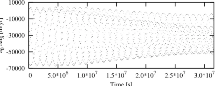
-70000 -50000 -30000 -10000 10000 5.0*106 1.0*107 1.5*107 2.0*107 2.5*107 3.0*107 a0 ∆ nS [m/yr] Time [s] 0
Fig. 3. Change of the mean motion due to the perturbation by the Sun.
-65 -30 5 40 5.0*106 1.0*107 1.5*107 2.0*107 2.5*107 3.0*107 a0 ∆ nD [m/yr] Time [s] 0
Fig. 4. Change of the mean motion due to the perturbation by Deimos.
-2 -0.5 1 2.5 4 5.0*106 1.0*107 1.5*107 2.0*107 2.5*107 3.0*107 a0 ∆ nJ [m/yr] Time [s] 0
Fig. 5. Change of the mean motion due to the perturbation by Jupiter.
-22 -17 -12 -7 -2 3 5.0*106 1.0*107 1.5*107 2.0*107 2.5*107 3.0*107 a0 ∆ nt [m/yr] Time [s] 0
Fig. 6. Change of the mean motion due to the perturbation by tide of
the Sun.
has been added to the right hand side of the equations, for ex-ample the perturbation by the Sun. In this way one can estimate the influence of the perturbation by the Sun into the change of the coordinates of Phobos. This estimation may be done after subtracting the influence of the change of the coordinates of Phobos caused by all the elements of the potential considered before adding the perturbation by the Sun. Such a procedure has been done for all the perturbations. The perturbations which have been rejected in the perturbational functionKpalso have been added to the right hand side of the EOMs in order to check ifKp(Eq. (34)) has been chosen correctly.
-150 -90 -30 30 90 150 5.0*106 1.0*107 1.5*107 2.0*107 2.5*107 3.0*107 a0 ∆ npr [m/yr] Time [s] 0
Fig. 7. Change of the mean motion due to the perturbation by
preces-sion. -1 -0.5 0 0.5 1 5.0*106 1.0*107 1.5*107 2.0*107 2.5*107 3.0*107 a0 ∆ nMVESUNP [m/yr] Time [s] 0
Fig. 8. Change of the mean motion due to the perturbation by Mercury,
Venus, Earth, Saturn, Uranus, Neptune and Pluto.
-2700 -1700 -700 300 5.0*106 1.0*107 1.5*107 2.0*107 2.5*107 3.0*107 a0 ∆ nj4 [m/yr] Time [s] 0
Fig. 9. Change of the mean motion due to the perturbation byj4.
-500 -300 -100 100 5.0*106 1.0*107 1.5*107 2.0*107 2.5*107 3.0*107 a0 ∆ nj5 [m/yr] Time [s] 0
Fig. 10. Change of the mean motion due to the perturbation byj5.
-200 -50 100 250 5.0*106 1.0*107 1.5*107 2.0*107 2.5*107 3.0*107 a0 ∆ nj6 [m/yr] Time [s] 0
Fig. 11. Change of the mean motion due to the perturbation byj6.
-100 -60 -20 20 60 5.0*106 1.0*107 1.5*107 2.0*107 2.5*107 3.0*107 a0 ∆ nj7 [m/yr] Time [s] 0
Fig. 12. Change of the mean motion due to the perturbation byj7.
-8 -4.5 -1 2.5 6 5.0*106 1.0*107 1.5*107 2.0*107 2.5*107 3.0*107 a0 ∆ nj8 [m/yr] Time [s] 0
Fig. 13. Change of the mean motion due to the perturbation byj8.
-3.5 -2 -0.5 1 2.5 5.0*106 1.0*107 1.5*107 2.0*107 2.5*107 3.0*107 a0 ∆ nj9 [m/yr] Time [s] 0
Fig. 14. Change of the mean motion due to the perturbation byj9.
-10 -5 0 5 10 5.0*106 1.0*107 1.5*107 2.0*107 2.5*107 3.0*107 a0 ∆ nj10 [m/yr] Time [s] 0
Fig. 15. Change of the mean motion due to the perturbation byj10.
-0.75 0 0.75 1.5 5.0*106 1.0*107 1.5*107 2.0*107 2.5*107 3.0*107 a0 ∆ nj11 [m/yr] Time [s] 0
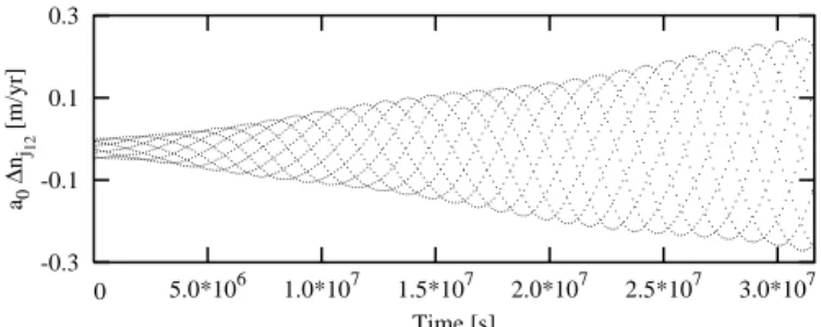
-0.3 -0.1 0.1 0.3 5.0*106 1.0*107 1.5*107 2.0*107 2.5*107 3.0*107 a0 ∆ nj12 [m/yr] Time [s] 0
Fig. 17. Change of the mean motion due to the perturbation byj12.
-0.6 -0.25 0.1 0.45 0.8 5.0*106 1.0*107 1.5*107 2.0*107 2.5*107 3.0*107 a0 ∆ nJ13 ...J 50 [m/yr] Time [s] 0
Fig. 18. Change of the mean motion due to the perturbation byj13...j50.
The values of the coordinates and of the velocity, evaluated with a step of two hours, have been used to estimate the mean motion of Phobos. The figures present the changes of the mean motion due to adding the specific components of the perturba-tional function to the right hand side of EOMs. The horizontal axis describes the time of the integration. The vertical axis de-scribes the change of the mean motion (∆n) of Phobos due to different perturbations multiplied by the value of the semi-major axis of the orbit of Phobosa0. The valuesa0∆nare expressed in meters over 1 year [m/yr]. Results are presented as points with a step of 2 hours for the period from0sto3.1×107s(1 year).
8. Conclusions
The numerical integration of the EOMs and analysis of the per-turbational function indicate that the terms of the perper-turbational function have been chosen correctly. Figs. 3-18 show the change of the mean motion of Phobos scaled bya0due to the perturba-tions by the Sun (a0∆nS), Deimos (a0∆nD), Jupiter (a0∆nJ), tide of the Sun (a0∆nt), precession (a0∆npr), Mercury, Venus, Earth, Saturn, Uranus, Neptune and Pluto (a0∆nMV ESUNP), j4...j50. Fig. 8 and Fig. 18 show those influences of the interac-tions with Phobos which may be negligible within the assumed precision. Mercury, Venus, Earth, Saturn, Uranus, Nep-tune, Pluto (see Fig. 8) and zonal harmonicsj13...j50(Fig. 18)
belong to this class of interactions. Changes of the mean mo-tion due to the perturbamo-tion by the Sun (Fig. 3), Deimos (Fig. 4), Jupiter (Fig. 5), tide of the Sun (Fig. 6), precession (Fig. 7), j4...j12 (Fig. 9-17) are large enough in order to be taken into account in this theory.
The Solar perturbations and the perturbations resulting from j4change the mean motion, respectively, of the order4×10−1 rad/yr and 2×10⁻²rad/yr. Zonal harmonicsj5...j12modify the mean motion, respectively, by approximately3×10−3,2×
10−3,8×10−4,6×10−5,3×−5,1×10−4,1×10−5,3×10⁻⁶ rad/yr. The tidal effects resulting from the interaction between Sun and Mars are of the order1×10−4rad/yr. Deimos, in spite of its small size, introduces perturbations in the mean motion of the order5×10−4rad/yr. Non-inertiality of the coordinate system as well as the interaction between Phobos and Jupiter lead to a change in the mean motion of the order1×10−3–
2×10⁻⁵rad/yr.
Hamiltonian in this case has been expressed as a polynomial containing about22 000terms.
The next step will be the analytical integration of the equa-tions of the motion. The work on this subject is in progress and will be published in a forthcoming paper.
Acknowledgements. This work has been supported by the Polish KBN,
project No. 2 PO3D 003 14. The author is indebted to Prof. A. Dro˙zyner for supplying the computer code.
References
Abad A., San-Juan J. F., 1994, In: Kurzy´nska K., Barlier F., Seidel-mann P.K., Wytrzyszczak I. (eds.) Dynamics and Astrometry of Natural and Artificial Celestial Bodies. Astronomical Observatory of A.M.U., Pozna´n, p. 383
Aksenov E.P., 1977, Theory of the Motion of Artificial Earth Satellite. Nauka, Moskwa
Born G.H., Duxbury T.C., 1975, Celest. Mech. 12, 77 Bretagnon P., 1982, A&A 114, 278
Chapront-Touz´e M., 1988, A&A 200, 255
Emelianov N.V., Nasonova L.P., 1984, AZh 61, 1021
Emelianov N.V., Vashkovyak S.N., Nasonova L.P., 1993, A&A 267, 634
Everhart E., 1974, Celest. Mech. 10, 35 Goldreich P., 1965, AJ 70, 5
Jacobson R.A., Synnott S.P., Campbell J.K., 1989, A&A 225, 548 Morley T.A., 1990, A&A 228, 260
Smith D.E., Lerch F.J., Nerem R.S., et al., 1993, J. Geophys. Res. Vol. 98, No. E11, 20, 871
Sinclair A.T., 1972, MNRAS 155, 249 Sinclair A.T., 1989, A&A 220, 321 Shor V.A., 1975, Celest. Mech. 12, 61 Shor V.A., 1988, Lett. AZh 14, 1123