A NEW ROOT–FINDING ALGORITHM USING EXPONENTIAL SERIES

(1)

A NEW ROOT-FINDING ALGORITHM USING

EXPONENTIAL SERIES

Srinivasarao Thota

Department of Applied Mathematics, School of Applied Natural Sciences, Adama Science and Technology University,

Post Box No. 1888, Adama, Ethiopia

Abstract:In this paper, we present a new root-finding algorithm to compute a non-zero real root of the tran-scendental equations using exponential series. Indeed, the new proposed algorithm is based on the exponential series and in which Secant method is special case. The proposed algorithm produces better approximate root than bisection method, regula-falsi method, Newton-Raphson method and secant method. The implementation of the proposed algorithm in Matlab and Maple also presented. Certain numerical examples are presented to validate the efficiency of the proposed algorithm. This algorithm will help to implement in the commercial package for finding a real root of a given transcendental equation.

Keywords:Algebraic equations, Transcendental equations, Exponential series, Secant method.

Introduction

The root finding algorithms are the most relevant computational problems in science, engineer-ing. The applications of root finding algorithms arise in many practical applications of Biosciences, Physics, Engineering, Chemistry etc. As mentioned in [1], the finding of any unknown appearing implicitly in engineering or scientific formulas, gives rise to root finding problem. A root of a functionf(x) is a number ‘α’ such thatf(α) = 0. Generally, the roots of transcendental functions cannot be expressed in closed form or cannot be computed exactly. The root-finding algorithms give us approximations to the roots, these approximations are expressed either as small isolating intervals or as floating point numbers. In the literature, there are several root finding algorithms are available, see for example, [1–11]. The basic root-finding methods are Bisection, False position, Newton-Raphson, Secant methods etc. Most of the algorithms use iteration, producing a sequence of numbers that hopefully converge towards the root as a limit. The rates of converge of different algorithms are different. That is, some algorithms are faster converges to the root than others algo-rithms. The purpose of existing algorithms is to provide higher order convergence with guaranteed root. Many existing algorithms do not guarantee that they will find all the roots; in particular, if such an algorithm does not find any root, that does not mean that no root exists. There are many well known root finding algorithms available to find an approximate root of algebraic or transcendental equations., see for example, [1,5,6,8, 9,11].

(2)

discuss some numerical examples to illustrate the algorithm and comparisons are made to show efficiency of the new algorithm.

1. New algorithm using exponential series

The new iterative formula using exponential series is proposed as follows, for any two initial approximations x0, x1 of the root,

xn+1 =xnexp

xn−₁f(xn)−xnf(xn)

xnf(xn)−xnf(xn−₁)

, n= 1,2, . . . . (1.1)

By expanding this iterative formula, one can obtain the standard secant method as in first two terms, and many methods are obtained based on series truncation. Indeed,

xn+1=xn−

f(xn)(xn−xn−₁)

f(xn)−f(xn−₁)

. (1.2)

xn+1 =xn−

f(xn)−f(xn−₁)

+ 1 2xn

f(xn)−f(xn−₁)

2

. (1.3)

xn+1 =xn−

f(xn)−f(xn−₁)

+ 1 2xn

f(xn)−f(xn−₁)

2

− 1 6x2

n

f(xn)−f(xn−₁)

3

. (1.4)

This is shown in the following theorem.

Theorem 1. Supposeα₆= 0 is a real exact root of f(x) andθis a sufficiently small neighbour-hood of α. Let f′′

(x) exist and f′

(x) ₆= 0 in θ. Then the iterative formula given in equation (1.1) produces a sequence of iterations _{xn:n= 1,2,3, . . .} with order of convergencep≥(1 +

√ 5)/2. P r o o f. The iterative formula given in equation (1.1) can be expressed in the following form

xn+1 =xnexp

.

Since

lim

xn→α

exp

= 1, and hencexn+1 =α.

Using the standard expansion of ex

as exp(x) = 1 +x+1

2x

2₊1

6x

3₊ 1

24x

4₊_{· · ·} _(1.5)

and from equations (1.1) and (1.5), we have

xn+1=xnexp

=xn(1 +

+ 1 2

2

+1 6

3

+_{· · ·})

=xn−

f(xn)−f(xn−₁)

+ 1 2xn

f(xn)−f(xn−₁)

2

−₆_x1₂

n

f(xn)−f(xn−₁)

3

+o 1 24x3

n

f(xn)−f(xn−₁)

4!

(3)

Sincef(xn)≈0, when we neglect higher order terms, then the above equation gives secant method

in first two terms. Indeed, we have the following formulae obtained from first two terms, three terms and four terms of the expansion respectively as given in equations (1.2)–(1.4).

xn+1=xn−

f(xn)−f(xn−₁)

.

xn+1 =xn−

f(xn)−f(xn−₁)

+ 1 2xn

f(xn)−f(xn−₁)

2

.

xn+1 =xn−

f(xn)−f(xn−₁)

+ 1 2xn

f(xn)−f(xn−₁)

2

−₆_x1₂

n

f(xn)−f(xn−₁)

3

.

In the above equations, we obtained secant method having (1 +√5)/2 convergence in first two terms. Therefore, the order of convergence of proposed methods (1.1), (1.3) and (1.4) are at least

p_≥(1 +√5)/2.

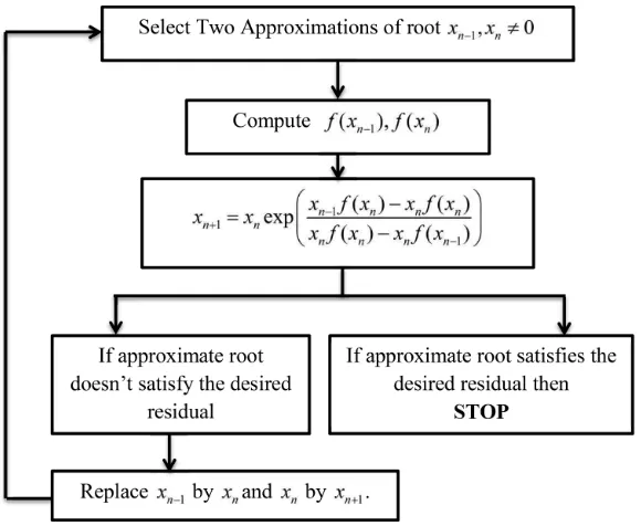
1.1. Steps for computing root

I. Select two approximations x0 andx16= 0.

II. Compute f(x0) and f(x1).

III. Compute the next approximate root using formula given in (1.1).

IV. Repeat Step II and III until we get desired approximate root.

Flow chat of the proposed algorithm is presented in Figure 1.

(4)

2. Implementation of proposed algorithm

2.1. Proposed algorithm in MATLAB

In this section present MATLAB implementation of the proposed algorithm as follows.

a=input(’Given Function:’,’s’);

f=inline(a); % Given function is storing in f

x(1)=input(’Enter x0: ’); % Initial approximation x0

x(2)=input(’Enter x1: ’); % Initial approximation x1

n=input(’Enter Allowed Error: ’); % n is allowed error

iteration=0;

for i=3:1000

x(i) = x(i-1)*exp((x(i-2)*f(x(i-1))-x(i-1)*f(x(i-1)))/ (x(i-1)*f(x(i-1))-x(i-1)*f(x(i-2))));% main eq (1.1)

iteration=iteration+1;

if abs((x(i)-x(i-1))/x(i))*100<n root=x(i)

iteration=iteration

break % breaking if abs error_≥n

end end

Sample computations using the implementation of the proposed algorithm are presented in Sec-tion 3.

2.2. Proposed algorithm in MAPLE

In this section, we provide the implementation of the proposed method in Maple as follows. To execute the maple code, one should enter the required date attypetext.

eps step := type; eps abs := type; f(x):= type; x[0] := type; x[1] := type; n:= type;

for i from 2 to n do

printf("Iteration No: %g", i-1);

x[i] := x[i-1]*exp((x[i-2]*f(x[i-1])-x[i-1]*f(x[i-1]))/ (x[i-1]*f(x[i-1])-x[i-1]*f(x[i-2])));

if abs(x[i]-x[i-1]) < eps step and abs(f(x[i])) < eps abs then break;

(5)

Sample computations using the implementation of the proposed algorithm are presented in Sec-tion 3.

3. Numerical examples

This section provides some numerical examples to discuss the algorithm presented in Section1

and comparisons are taken into account to conform that the algorithm is more efficient than other existing methods.

Example 3.1. Consider an equation

x6₋x₋1 = 0. (3.1)

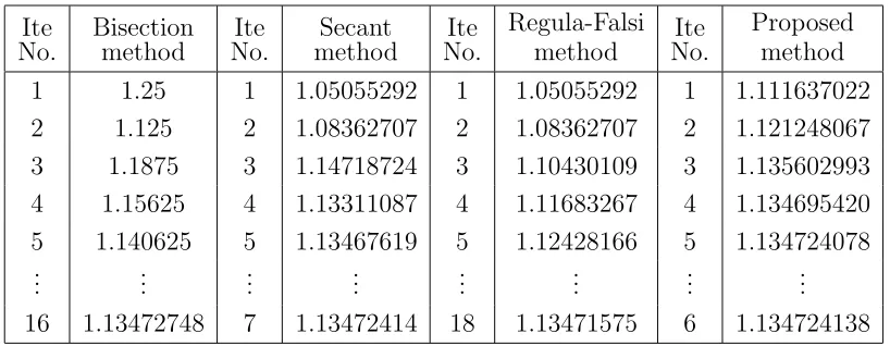
This equation has two real roots ₋0.7780895987 and 1.134724138. The following Table 1 shows the comparison between various existing methods and proposed method at accurate to within ǫ= 0.00001 with initial approximations x0 = 1 andx1= 1.5.

Table 1. Comparing approximate root using various existing methods

Ite

No. Bisectionmethod No.Ite methodSecant No.Ite

Regula-Falsi method No.Ite

Proposed method 1 1.25 1 1.05055292 1 1.05055292 1 1.111637022 2 1.125 2 1.08362707 2 1.08362707 2 1.121248067 3 1.1875 3 1.14718724 3 1.10430109 3 1.135602993 4 1.15625 4 1.13311087 4 1.11683267 4 1.134695420 5 1.140625 5 1.13467619 5 1.12428166 5 1.134724078

... ... ... ... ... ... ... ... 16 1.13472748 7 1.13472414 18 1.13471575 6 1.134724138

One can observe from the Table1 that the proposed algorithm gives approximate root quicker than the other existing methods.

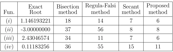
Example 3.2. Consider the following transcendental equations. We compare the number of iterations required to get approximation root. The numerical results are provided in Table2.

(i) f(x) =ex

−x₋2, with initial approximation 1 and 2 with accuracy of 10−₅

.

(ii) f(x) = 2x3+ 11x2+ 12x₋9, with initial approximations₋5 and₋1 with accuracy of 10−₁₀

. (iii) f(x) = 8₋4.5(x₋sinx), with initial approximations 2 and 3 with accuracy of 10−₁₀

. (iv) f(x) =xe−x

−0.1, with initial approximation ₋0.9 and 0.9 with accuracy of 10−₁₀

.

The numerical results given in Table 2 shows that the proposed method is more efficient than other methods.

Example 3.3. Recall the Example 3.1 for the sample computations using Matlab and Maple implementation as described in Section 2.

(6)

Table 2. Comparing No. of iterations by different methods

Fun. ExactRoot Bisectionmethod

Regula-Falsi

method methodSecant

Proposed method (i₎ _1.146193221 ₁₈ ₁₄ ₇ ₆ (ii₎ _-3.00000000 ₃₇ ₅₆ ₈ ₈ (iii₎ _2.43046574 ₃₄ ₁₁ ₇ ₆ (iv₎ _0.11183256 ₃₆ ₅₅ ₁₅ ₁₁

with initial approximations 1 and 1.5.

Using Matlab implementation, we have the following computations.

>> ExpSecant Given Function:x∧

6-x-1 Enter x0: 1.0

Enter x1: 1.5

Enter Allowed Error: 0.00001 root=

1.1347

iteration=

6

Using Maple implementation, we have the following computations.

> eps step := 1e-5: > eps abs := 1e-5: > f(x):= x∧

6-x-1: > x[0] := 1.0: > x[1] := 1.5: > n:= 100:

> for i from 2 to n do

> printf("Iteration No: %g", i-1);

> x[i] := x[i-1]*exp((x[i-2]*f(x[i-1])-x[i-1]*f(x[i-1]))/ (x[i-1]*f(x[i-1])-x[i-1]*f(x[i-2])));

> if abs(x[i]-x[i-1]) < eps step and > abs(f(x[i])) < eps abs then

(7)

Iteration N o: 1

1.111637022 Iteration N o: 2

1.121248067 Iteration N o: 3

1.135602993 Iteration N o: 4

1.134695420 Iteration N o: 5

1.134724078 Iteration N o: 6

1.134724138

One can use the implementation of the proposed algorithm to speed up the manual calculations.

4. Conclusion

In this work, we presented a new algorithm to compute an approximate root of a given transcen-dental function better than previous existing methods as illustrated. The proposed new algorithm was based on exponential series having better convergence than previous existing methods(for ex-ample, Bisection, Regula–Falsi, Secant methods etc.). This proposed algorithm is useful for solving the complex real life problems. Implementation of the proposed algorithm in Matlab and Maple is also discussed presented sample computations.

Acknowledgment

The author is thankful to the editor and reviewers for providing valuable inputs to improve the present format of manuscript.

REFERENCES

1. Datta B. N. Lecture Notes on Numerical Solution of Root–Finding Problems. 2012. URL:http://www.math.niu.edu/ dattab/math435.2009/ROOT-FINDING.pdf.

2. Chen J. New modified regula falsi method for nonlinear equations.Appl. Math. Comput., 2007. Vol. 184, No. 2. P. 965–971.DOI: 10.1016/j.amc.2006.05.203

3. Noor M. A., Noor K. I., Khan W. A., Ahmad F. On iterative methods for nonlinear equations. Appl. Math. Comput., 2006. Vol. 183, No. 1. P. 128–133.DOI: 10.1016/j.amc.2006.05.054

4. Noor M. A., Ahmad F. Numerical comparison of iterative methods for solving nonlinear equations.Appl. Math. Comput., 2006. Vol. 180, No. 1. P. 167–172.DOI: 10.1016/j.amc.2005.11.151

5. Ehiwario J. C., Aghamie S. O. Comparative study of bisection, Newton-Raphson and secant methods of root–finding problems.IOSR J. of Engineering, 2014. Vol. 4, No. 4. P. 1–7.

(8)

8. Thota S., Srivastav V. K. Quadratically convergent algorithm for computing real root of non-linear tran-scendental equations.BMC Research Notes, 2018. Vol. 11, art. no. 909.DOI: 10.1186/s13104-018-4008-z 9. Thota S., Srivastav V. K. Interpolation based hybrid algorithm for computing real root of non-linear transcendental functions. Int. J. Math. Comput. Research, 2014. Vol. 2, No. 11, P. 729–735. URL:http://ijmcr.in/index.php/ijmcr/article/view/182/181

10. Abbasbandy S., Liao S. A new modification of false position method based on homotopy analysis method.

Appl. Math. Mech., 2008. Vol. 29, No. 2. P. 223–228.DOI: 10.1007/s10483-008-0209-z