Stationarity and cointegration tests: Comparison of Engle Granger and Johansen methodologies

Munich Personal RePEc Archive

Stationarity and cointegration tests:

Comparison of Engle - Granger and

Johansen methodologies

Bilgili, Faik

Erciyes University, Faculty of Economics and Administrative

Sciences

1998

Online at

https://mpra.ub.uni-muenchen.de/75967/

1

STATIONARITY AND COINTEGRATION TESTS: COMPARISON OF ENGLE - GRANGER AND JOHANSEN METHODOLOGIES

Faik Bilgili

Abstract

Engle-Granger methodology follows two-step estimations. The first step generates the residuals and the second step employs generated residuals to estimate a regression of first-differenced residuals on lagged residuals. Hence, any possible error from the first step will be carried into second step.

The Johansen maximum likelihood methodology circumvents Engle-Granger methodology by estimating and testing for the presence of multiple cointegrating vectors through largest canonical correlations. The number of non-zero eigenvalues of Ψ of eq. 26 in the text will specify the number of cointegrating vectors. Some Monte Carlo evidence explores that Johansen procedure performs better than both single equation methods and alternative multivariate methods. In fact, evidence of this paper reveals, as well, that, as Engle-Granger yields some inconclusive outcome, the Johansen tests reach at least one cointegration relationship among variables for Canada, India, Italy, Japan, Turkey and the USA. Then, one may claim that Johansen methodology dominates the Engle- Granger methodology in cointegration analyses.

I. INTRODUCTION

Macroeconomic time series studies are based on the assumption that the underlying time series is stationary. Time series studies, however, show that many time series are not stationary in their levels but stationary in differences. The results of regression a nonstationary time series variable on another nonstationary time series variable yields often spurious results although there is no meaningful relationship between them.

To avoid spurious results such as biased traditional F and t statistics, one should use stationary variables in their levels or difference stationary variables. Stationarity

means that the time series has a constant mean, m and finite (bounded) variance, σ2.

2

Section II explains relationship between stationarity and cointegration. In section III, two methodologies for testing cointegration, Engle-Granger and Johansen methodologies, show the testing procedures for cointegration step by step. Section IV gives empirical evidence on cointegration by comparing Engle-Granger and Johansen methodologies.

II. STATIONARITY AND COINTEGRATION

Test for unit roots are performed on univariate time series. Considering the univariate time series in eq. (1),

𝑦

𝑡∗

= Ϛ𝑦

𝑡−1∗

+ 𝑢

𝑡

.

(1)

where y*t is measured as deviations of y from its population mean, u. Expected value

of random error is equal to zero, E(ut} = 0 and variance of random error is zero finite

(a scalar),

Var (u

t

) = σ

2

, or, E[u

t

–

E(u

t

)]

2

= σ

2

Consider now the multivariate time series,

𝑿

𝒕

= Ф

𝟏

𝑿

𝒕−𝟏

+ Ф

𝟐

𝑿

𝒕−𝟐

+ Ф

𝟑

𝑿

𝒕−𝟑

+ ⋯ + Ф

𝒑

𝑿

𝒕−𝒑

+ 𝒆

𝒕

.

(2)

where Ф_𝑝 𝑋_𝑡−𝑝 is n-by-n matrix. Eq. (2) can be reparameterized as

∆𝑿

_𝒕

= П

_𝟏

∆𝑿

_𝒕−𝟏

+ П

_𝟐

∆𝑿

_𝒕−𝟐

+ ⋯ + П

_𝒑−𝟏

∆𝑿

_{𝒕−𝒑+𝟏}

− Ф

𝑿

_𝒕−𝟏

+ 𝒆

_𝒕

.

(3)

In eq. (1), if σ =0, yt is known as random walk or nonstationary time series.

In eq. (3), if the matrix Φ = ( I - Φ1 - Φ2 - Φ3 - .... Φp ) is full rank, then any linear

combination of xt will be stationary. The test for cointegration is to test for rank of Φ

by testing whether the eigenvalues of estimated Φ are significantly different from

zero.

Studies of macroeconomic theory assume that there should be a stable long-run

relationship among variables. İn the existence of long-run relationship, variables

cannot move too far from each other. If individual time series are not stationary, they can wander too far from each other, and traditional statistics of a projection of one

nonstationary variable on another become unreliable1. lf series are stationary but

cointegrated, however, they are expected to move together in the long-run. in short, cointegration means that one or more linear combinations of these variables is stationary even though individually they are not.

1

3

III. COINTEGRATION TESTS BY ENGLE-GRANGER AND JOHANSEN

METHODOLOGIES

In this section, I will first introduce theorems and then explain the statistical calculations of the Engle-Granger and Johansen tests. In fact, there are several estimations of cointegration relations, such as, OLS (Engle-Granger, 1987), Augmented Least Squares (Bewley, 1979; Hendry and Richard, 1982), Instrumental Variables (Phillips and Hansen, 1990), Fully Modified Estimator (Park and Phillips, 1988), Non-Parametric Canonical Cointegration (Park, 1989), Three Step Estimator (Engle and Yoo, 1991), Canonical Cointegration (Bossaerts, 1988), Spectral Regression (Phillips, 1991), Principal Components (Stock and Watson, 1989), Maximum Likelihood (Johansen, 1988), Modified Box-Tiao (Bewley, Orden and

Fisher, 1991)2. In this study, however, I examine the two of them, Engle- Granger and

Johansen procedures, since they have been the most commonly used among others for cointegration analyses. The OLS estimator is the simplest one to analyze the cointegration analysis while Maximum likelihood estimator is the best if the model is well specified without highly autocorrelated cointegrating errors.

III.1 Engle-Granger Methodology

Testing for cointegration by Engle-Granger methodology proposes a straightforward

test whether variable in xt vector are cointegrated. Let yt and zt be two variables in xt

vector and suppose they are integrated of order 1. Engle and Granger methodology

tests whether yt and zt are cointegrated of order CI(1,1).

Definition: The components of the vector xt are said to be cointegrated of order d, b,

denoted

xt ~ CI(d,b), if

a- all components of xt are I (d),

b- there exists a vector b (≠ 0) so that m = b’xt ~ I (d~b), b > 0. The vector b is called

the co-integrating vector3.

One can perform Engle-Granger cointegration test as follows4:

1- Determine order of integration of variables yt and zt. If they are integrated of the

same order, one can apply the cointegration test. Eq. (1) can be tested for both yt and

zt by Dicky-Fuller or Augmented Dicky-Fuller to see if Ϛ = 0 for each variable. If it is

so, it would mean that variables are not stationary and that their differences might be integrated of order zero.

2

See Hargreaves (1994).

3

Engle and Granger (1991, p.84).

4

4

∆

y

t

= a

0

+

Ϛ

y

t-1

+ e

t

.

(4)

∆

y

t

= a

0

+

Ϛ

y

t-1

+ a

1

t + e

t

.

(5)

∆

2

_y

_t

_{= b}

₀

₊

Ϛ∆

_y

_t-1

_{+ e}

_t

_.

₍₆₎

∆

2

_y

_t

_{= b}

₀

₊

Ϛ∆

_y

_t-1

_{+ b}

₁

_{t + e}

_t

_.

₍₇₎

∆

3

_y

_t

_{= c}

₀

₊

Ϛ∆

2

_y

_t-1

_{+ e}

_t

_.

₍₈₎

∆

3

_y

_t

_{= c}

₀

₊

Ϛ∆

2

_y

_t-1

_{+ c}

₁

_{t + e}

_t.

_.

₍₉₎

∆

d

_y

_t

_{= m}

₀

₊

Ϛ∆

d-1

_y

_t-1

_{+ y}

_t-1

_{+ e}

_{t .}

₍₁₀₎

∆

d

_y

_t

_{= m}

₀

₊

Ϛ∆

d-1

_y

_t-1

_{+ y}

_t-1

_{+ m}

₁

_{t + e}

_t

_.

₍₁₁₎

The tests for eqs. (4) and (6) are Dicky-Fuller tests and the tests for eqs. (5) and (7)

are Dicky-Fuller with trend variable tests. One can write the same equations for zt as

well. The error term et is white noise, if it is serially uncorrelated and if its expected

mean is equal to zero. If et does not seem to be white noise, an Augmented Dicky

Fuller (ADF) test will be implemented. The number of lags of ADF is increased until et

becomes white noise. If Ϛ = 0 from eqs. (6) and (7) for each variable, then they are

integrated of order one, /(1), A series that needs to be differenced d times to achieve

stationary is said to be integrated of order d [ /(d)].

2-If the variables are found integrated of order one at first step, one can proceed the

following regressions and save the residuals.

y

t

= a

0

+ a

1

z

t

+ e

1,t

,

(12)

z

t

= b

0

+ b

1

y

t

+ e

2,t

.

(13)

3-Regress the following regressions and test for unit root for each equation.

∆

e

1t

= a

1

e

1t-1

+ v

1,t

,

(14)

∆

e

2t

= a

2

e

2t-1

+ v

2,t

.

(15)

If it is not possible to reject the null hypotheses that |a1| = 0 and |a2|= 0, one cannot

reject the hypothesis that the variables are not cointegrated.

III.2 Johansen Methodology

5

any r ≤ p, H0: rank(Φ) ≤ r or Φ = α B’, where α and B are pxr matrices. If there is

cointegration among variables, xt is cointegrated with the cointegration vectors B (Φ =

αB’).

One cannot estimate the parameters of α and B but can estimate the space spanned

by B.

Now, in estimation of space spanned by B, the theorem is as follows:

Theorem: The maximum likelihood estimator of the space spanned by B is the space spanned by the r canonical variates corresponding to the r largest squared canonical

correlations between the residuals of xt-p and ∆xt corrected for the effect of the lagged

differences of the x process5.

One can obtain the largest canonical correlation as follows6:

1-After determining the order of p, regress ∆xt on ∆xt-1 + ∆xt-2 + ∆xt-3 + ...+ ∆xt-p+1

and save the residuals.

2-Regress xt-p on ∆xt-1 + ∆xt-2 +∆xt-3 + ... + ∆xt-p+1 and save the residuals.

3-Let nt be residuals from step 1 and vt be residuals from step 2.

4-Compute squares of the canonical correlations7 between nt and vt as:

𝛀

_𝟏𝟐

> 𝛀

_𝟐𝟐

> 𝛀

_𝟑𝟐

> ⋯ > 𝛀

_𝐩𝟐

.

5-Maximal eigenvalue test that uses (r +1)th largest squared canonical correlation is

𝛀 𝐦𝐚𝐱 (𝐫, 𝐫 + 𝟏) = −𝑻𝒍𝒏 (𝟏 − 𝛀̂

_𝒓+𝟏𝟐

).

6-Or, one can obtain the trace test as follows:

𝛀 𝐭𝐫𝐚𝐜𝐞 (𝐫) = −𝑻 ∑

𝒏_{𝒊=𝒓+𝟏}

𝒍𝒏

(𝟏 − 𝛀̂

_𝒊𝟐

).

Ω trace and Ω max test the number of eigenvalues, r, that are statistically different

from zero: For instance, in the three-variable case, n = 3, Ω, trace tests the

hypothesis that there is no cointegration, against alternative that there are 1, 2, or 3

cointegration vectors. If H0: r = 0 is rejected against H1: r > 0, then H0: r < 1 is tested

against hypothesis r = 2 or 3. The Ω max is more specific than the Ω trace test,

whose null hypothesis is that there are no cointegrating vectors against the

hypothesis that there is one cointegrating vector. Or in Ω max tests; Ho: r =1 vs H1: r

=2, H0: r = 2 vs H1: r = 3.

5

S. Johansen (1988, p.234).

6

Dickey, Jansen and Thornton (1991, pp. 62-63).

7

6

IV. EMPIRICAL EVIDENCE

In this section, I will conduct all necessary tests indicated in section III for the variables of a basic consumption function below.

C

t

= a

0

+ a

1

Y

t

+ a

2

T

t

+ e

t

.

(18)

where C is real consumption, Y is real GDP and T is real tax revenues. Real consumption is a function of real income and taxes. It has been known from the literature that this function (or its slightly different version) has been tested recurrently to understand the consumption behavior. The basic concern is here, however, not to perform this regression indicated by eq.(18) but to see if one can use these variables in the model to estimate the aggregate demand. In other words, obtaining parameter estimates from this model is the second step which is not of interest here in this study. The purpose is to perform the first step which is to conduct the stationary tests and cointegration tests by Engle-Granger and Johansen methodologies.

These tests will be performed for seven countries; Canada, Germany, India, Italy, Japan, Turkey and the USA. Annual Private Consumption and GDP data were drawn from World Bank Data CD-ROM 1995 for the period 1960 to 1993. The Tax Revenues data were drawn from World Bank Data CD-ROM 1995 and IFS CD-ROM 1995 for the period 1970 to 1993. Nominal annual values were divided by the GDP

deflator to obtain real values of Ct, Yt, and Tt. The lag number = 4 was determined for

these countries by Akaike information criterion (AIC), and Schwartz Bayesian Criterion (SBC).

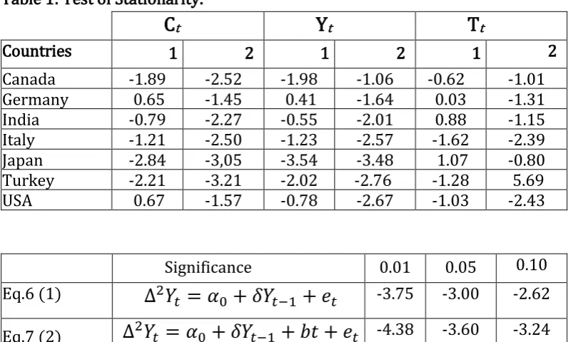
In Table 1, all Dicky-Fuller test results indicate that all variables for each country are

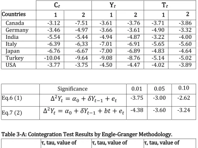
nonstationary except, Yt (by DF test without trend) of Japan. Table 2 shows that all

nonstationary variables are integrated of order one. Tables 3-A and 4-A give the results of cointegration tests by Engle-Granger and Johansen methodologies, respectively. Engle-Granger cointegration test can be run by eq.(19) through eq.(24).

C

t

= a

0

+ a

1

Y

t

+ a

2

T

t

+

e

1t

.

(19)

Y

t

= b

0

+ b

1

T

t

+ b

2

C

t

+ e

2t

.

(20)

T

t

= c

0

+ c

1

Y

t

+ c

2

C

t

+ e

3t

.

(21)

∆ε

1t

= α

1

ε

1t-1

+

v

1t

.

(22)

∆ε

2t

= α

2

ε

2t-1

+

v

2t

.

(23)

7

All residuals seem to be white noise, that is, null hypothesis that their means are equal to zero and that they are serially uncorrelated are all accepted at 0.05 levels. Therefore I did not run ADF tests for residuals. The cointegration results of eqs (22), (23) and (24) are given in Table 3-A. Tables 3-A and 3-B show that there exists no cointegration relation among variables of Canada, India and Japan

equations and that α3 of Germany, α2 of Italy and USA equation are statistically

significant, therefore there happens to be cointegration relation among the variables

in these countries. However α1 and α2 of Germany, α1 and α3 of Italy and the USA

equations do not confirm these cointegration results. Results are inconclusive. Under these inconsistent results, one may run Johansen cointegration test.

∆𝑿

𝒕

= 𝒄 + (Ф − 𝑰)𝑿

𝒕−𝟏

+ ∑

𝒑−𝟏𝒊=𝟏

Г

𝒊

∆𝑿

𝒕−𝒊

+ 𝒆

𝒕

.

(25)

∆𝑿

𝒕

= 𝒄 + 𝜳𝑿

𝒕−𝟏

+ ∑

𝒑−𝟏𝒊=𝟏

Г

𝒊

∆𝑿

𝒕−𝒊

+ 𝒆

𝒕

.

(26)

Where Г_i= (П₁+ П₂+ П₃+…+ П_p-1

),

Ф is an nxn matrix of parameters and I is an nxn

identity matrix. Eq. (26) is same as eq. (3). The number of non-zero eigenvalues of Ψ

will determine the number of cointegrating vectors. I apply the Johansen methodology that determines the number of non-zero eigenvalues by maximum likelihood method. One or more liner combinations of these variables might be stationary whereas

variables in Xt are non-stationary in levels as we see from Tables 1 and 2. The

[image:8.595.70.472.458.698.2]

eigenvalues of Ψ are given in Table 4-A.

Table 1: Test of Stationarity.

C

t

Y

t

T

t

Countries 1 2 1 2 1 2

Canada -1.89 -2.52 -1.98 -1.06 -0.62 -1.01

Germany 0.65 -1.45 0.41 -1.64 0.03 -1.31

India -0.79 -2.27 -0.55 -2.01 0.88 -1.15

Italy -1.21 -2.50 -1.23 -2.57 -1.62 -2.39

Japan -2.84 -3,05 -3.54 -3.48 1.07 -0.80

Turkey -2.21 -3.21 -2.02 -2.76 -1.28 5.69

USA 0.67 -1.57 -0.78 -2.67 -1.03 -2.43

Significance 0.01 0.05 0.10

Eq.6 (1)

∆

2

𝑌

_𝑡

= 𝛼

₀

+ 𝛿𝑌

_𝑡−1

+ 𝑒

_𝑡 -3.75 -3.00 -2.62

Eq.7 (2)

∆

2

𝑌

𝑡

= 𝛼

0

+ 𝛿𝑌

𝑡−1

+ 𝑏𝑡 + 𝑒

𝑡 -4.38 -3.60 -3.24

8

Furthermore, max and trace tests reveal that there are two cointegrating vectors in Canada, India and the USA equations and that there three cointegrating vectors appear in Italy, Japan and Turkey equations.

Table 2: Test of Integration.

C

t

Y

t

T

t

Countries 1 2 1 2 1 2

Canada -3.12 -7.51 -3.61 -3.76 -3.71 -3.86

Germany -3.46 -4.97 -3.66 -3.61 -4.90 -3.32

India -5.54 -5.44 -4.94 -4.87 -3.22 -4.00

Italy -6.39 -6,33 -7.01 -6.91 -5.65 -5.60

Japan -6.76 -6.67 -7.00 -6.89 -4.83 -4.64

Turkey -10.04 -9.64 -9.08 -8.76 -5.14 -5.02

USA -3.77 -3.75 -4.50 -4.47 -4.02 -3.89

Significance 0.01 0.05 0.10

Eq.6 (1)

∆

2

𝑌

_𝑡

= 𝛼

₀

+ 𝛿𝑌

_𝑡−1

+ 𝑒

_𝑡 -3.75 -3.00 -2.62

[image:9.595.68.472.152.453.2]

Eq.7 (2)

∆

2

𝑌

𝑡

= 𝛼

0

+ 𝛿𝑌

𝑡−1

+ 𝑏𝑡 + 𝑒

𝑡 -4.38 -3.60 -3.24

Table 3-A: Cointegration Test Results by Engle-Granger Methodology.

Countries

τ, tau, value of α1

τ, tau, value of

α2

τ, tau, value of

α3

Canada 1.24 1.74 2.05

Germany 3.38 1.93 3.73

India 3.09 3.16 3.19

Italy 3.63 9.85 2.36

Japan 3.32 3.31 0.03

Turkey 5.56 6.11 4.86

USA 3.54 3.88 3.36

Table 3-B: Critical Values for Cointegration tests by Engle and Yoo8_.

0.01 0.05 0.10

4.84 4.11 3.73

8

9

Table 4-A: Cointegration Test Results by Johansen.

Countries

λ

_i

λ

_Max

λ

_Trace

λ1 = 0.8539 32.70 53.61

Canada λ2 = 0.6743 19.07 20.90

λ3 = 0.1023 1.84 1.84 λ1 = 0.6815 21.74 31.09

Germany λ2 = 0.3272 7.53 9.35

λ3 =0.0914 1.82 1.82 λ1 = 1.0000 405.57 443.17

India λ2 =0.9170 37.33 37.60 λ3 = 0.0179 0.27 0.27 λ1 = 0.9998 134.22 182.86

Italy λ2 = 0.8829 34.31 48.64 λ3 = 0.5915 14.32 14.32

λ1 = 0.9220 43.36 78.45

Japan λ2 = 0.7512 23.65 35.10

λ3 = 0.4901 11.45 11.45

λ1 = 0.9408 53.70 91.35

Turkey λ2 =0.7884 29.51 37.65

λ3 = 0.3483 8.14 8.14

λ1 = 0.9495 50.76 73.04

USA λ2 = 0.7029 20.63 _22.28

λ3 = 0.0924 1.65 1.65

Table 4-B: NuII and Alternative Hypotheses by Johansen Methodology.

λ Trace Test

λ Max Test

H0: H1: H0: H1:

r = 0 r > 0 r= 0 r = 1

r ≤ 1 r > 1 r = 1 r = 2

r ≤ 2 r > 2 r = 2 r = 3

Table 4-C: Critical Values for λ Max and λ Trace tests9_.

n-r

λ Max

λ Trace

0.10 0.05 0.01 0.10 0.05 0.01

1 7.56 9.09 12.74 7.56 9.09 12.74

2 13.78 15,75 19.83 17.95 20.16 24.98

3 19.79 21.89 26.40 32.09 35.06 40.19

9

10

V. CONCLUSION

Many economic theories imply that a linear combination of variables is stationary although individually they are not. If there is such a stable linear combination among variables, the variables are said to be cointegrated. In existence of cointegration or long-run relationship, the variables have the same stochastic trends and therefore they cannot drift too far apart. In time series analysis of macroeconomic studies, hence, one should check for stationarity and cointegration to avoid losing long term information.

There are several methods in examining the cointegration analyses. Engle- Granger and Johansen procedures are the most commonly used among others in the literature. In Engle-Granger procedure, one examines the residuals from long-run equilibrium relationship by ordinary least squares method. The variables are cointegrated if these residuals do not yield unit root. Johansen procedure, in estimation cointegration relationship, estimates a vector autoregression in first differences and includes the lagged level of the variables in some period t-p.

There are several problems of Engle-Granger methodology. First, in examining residuals from the long-run equation relationship, there is no presumption that any of the, for instance, three residual series in three-variable case, is preferable to any of the others. One can find a cointegration relationship from residuals of the first regression whereas residuals of second and the third regressions may not yield a cointegration result. In other words, in finite sample case, the test for unit root in the error term sequence from the first regression may not be equivalent to the test for unit root in the error term sequence from another regression. Indeed, results of Section IV confirm this problem.

Engle-Granger methodology relies on a two-step estimator. The first step is to generate the residuals and the second step uses these generated residuals to estimate a regression of first-differenced residuals on lagged residuals. Therefore any error occurred in the first step will be carried into second step.

11

BIBLIOGRAPHY

Dickey, David A. and Jansen W. Dennis, Thornton L, Daniel, "A Primer on

Cointegration with an Application to Money and Income”, Federal Reserve Bank of St

Louis, March/April, 1991.

Enders, Walter, Applied Econometric Time Series, John Wiley & Sons, Inc., New York, 1995.

Engle, R. and C. Granger, "Cointegration and Error Correction:

Representation, Estimation, and Testing,” In Engle and Granger (eds.), Long Run

Economic Readings in Cointegration, Oxford University Press, New York, 1991, 81-113.

Engle, R. and Yoo Sam, "Forecasting and Testing in Co-integrated Systems," In Engle and Granger (eds.), Long Run Economic Relationships. Readings in Cointegration, Oxford University Press, New York, 1991, 237-67.

Granger, Clive, "Developments in The Study of Cointegrated Economic Variables," In Engle and Granger (eds.), Long Run Economic Relationships, Readings in Cointegration, Oxford University Press, New York, 1991,65-81.

Granger, Clive and P. Newbold, "Spurious Regressions in Econometrics,”

Journal of Econometrics, 2 (1974), 111-20.

Hamilton, James D, Time Series Analysis, Princeton University Press, Princeton, New Jersey, 1994.

Hargreaves, Colin, "A Review of Methods of Estimating Cointegrating

Relationships,” In Colin P. Hargreaves (ed.), Nonstationary Time Series Analysis and

Cointegration, Oxford University Press, New York, 1994, 87-133.

Johansen, Soren, "Statistical Analysis of Cointegration Vectors," Journal of Economic Dynamics and Control, 12 (1988), 231-254.

Johansen, S. and K. Juselius, "Maximum Likelihood Estimation and Inference on Cointegration with Application to the Demand for Money," Oxford Bulletin of Economics and Statistics, 52 (1990), 169-209.