ISSN 2307-7743 http://scienceasia.asia
_______________
Key words and phrases: Tungiasis, Equilibrium states, Stability, Lyapunov function, numerical simulation. © 2017 Science Asia
1 / 24
STABILITY ANALYSIS OF THE DYNAMICS OF TUNGIASIS TRANSMISSION IN ENDEMIC AREAS
JAIROS KAHURU1,*, LIVINGSTONE LUBOOBI1,2, YAW NKANSAH-GYEKYE1
Abstract:
Tungiasis refers to the infestation caused by the permanent penetration of the female sand flea “Tunga penetrans” into the skin of the human or animal hosts and causes cutaneous lesion. In this paper, we developed a deterministic model for the dynamics of tungiasis in communities of human beings, animal reservoirs and flea infested environment in order to understand the way tungiasis disease spreads in a poor resource community. We established the conditions for local and global stability of the disease-free and endemic equilibrium points. The computational results showed that the disease-free equilibrium point is locally and globally asymptotically stable when the model basic reproduction number R0 is less than unit, that isR0 1. Using the Lyapunov stability theory and LaSalle’s
Invariant Principle we found that the endemic equilibrium point (EE) is globally asymptotically stable whenR0 1. The numerical simulations have been presented to illustrate the way the model variables behave when there is no intervention and that the endemic equilibria exist and they are stable. On-host and off-host control measures which include focal spraying of insecticides to the premises, application of insecticidal dusts on animal bodies, environmental and personal hygiene, educational campaign, use of closed foot wear and application of plant based repellents should be implemented.
1 Introduction
enter into decisions in a way that human reasoning and debate cannot (Bawa, 2013). Generally the disease dynamics requires a variety of mathematical tools, from model creation to solving differential equations to statistical analysis (Pathak et al., 2010).
The basic concept in mathematical modeling is stability analysis of the equilibria of the epidemic models. The method based on the use of stable Metzler matrices has been proposed and proven to be useful to establish the global stability of the disease free equilibrium as described by Kamgang and Sallet (2008). The importance of the Metzler matrices is well recognized in the stability of dynamical systems and positive systems, more generally in biology, engineering and economics (Gupta, et al., 2014). On the other hand Lyapunov Direct Method by Korobeinikov (2002, 2004, and 2007) and McCluskey, (2006) combined with LaSalle’s Invariance Principle (LaSalle, 1976) has been a powerful tool for the analysis of stability of autonomous systems of differential equations through construction of suitable Lyapunov functions. Lyapunov functions are developed to establish the global asymptotic stability of the endemic equilibrium points.
In this paper we consider the dynamics of tungiasis that involves the interaction between humans, animal reservoirs and flea contaminated environment. We determine the model equilibria and analyze their stability at local and global level. We establish the local stability of the disease-free equilibrium point using trace and determinant criterion, the global stability of the disease-free equilibrium point using stable Metzler matrix theory and we also establish the global stability of the endemic equilibrium point using Lyapunov direct Method combined with LaSalle’s Invariance Principle. Finally, we perform numerical simulations of the model system in a closed population to present the results. The rest of this paper is organized as follows. In the second section, we present the model with its basic properties. In the third section we carry out a qualitative analysis of the model whereby stability conditions for the disease-free equilibrium and the endemic equilibrium are derived. The fourth section presents different computer simulations of the system. In the last section, the biological significance of our analytical and numerical findings is discussed.
2 Materials and methods 2.1Model formulation
The total human population at any timet, denoted by NH is subdivided into three distinct
epidemiological subpopulations namely susceptible humansSH, people who are mildly
infested by jiggers IHl and the people who are severely infested by jiggersIHh. SH is
acquire infestation from the infested animal reservoir IAh and the flea infested environment FE following the force of infestationHand move to either IHl or IHh at the rates AH IAh NH and EHEHrFFE
kFE
respectively. IHl may acquire infestation from the environment as well and progresses into IHh at a rateEHEHrF FE
kFE
. We assume that individuals in classes SH and IHl suffer only natural death at a rate H and for classHh
I the individuals suffer both the natural death at a rate Hand disease induced death at a rateH. Similarly the animal reservoir population denoted by NA is subdivided into
three subpopulations namely, the susceptible animals reservoirs SA, animals that are
mildly infested by jiggers IAl and animals that are severely infested by jiggersIAh. SA is
generated through birth at a rate bA so that its recruitment rate is bANA. SAmay acquire
infestation from infested animal reservoir IAh and the flea infested environment FE
following the force of infestation A, and move to either IAl or IAh at the rates A
Ah AI N
and EAEArF FE
kFE
respectively. IAl may acquire infestation from the environment as well and progresses into IAh at a rateEAEArF FE
kFE
. We assume that individuals in classes SAand IAl suffer only natural death at a rateA and the individualsclass in IAh suffers both the natural death at a rate Aand disease induced death at a rateA. The sub-model of environmental component consists of larvae and adult fleas compartments denoted by LE and FErespectively. From within bodies of IHh and IAh eggs are shed by the gravid female flea into the environment at an average rate
e with contribution rates of
eIHh and
eIAh respectively so that they hatch and mature into adult fleas. The compartment LE suffers a natural mortality rate L and matures to adult fleasclass FE at a rate L. At class FE the fleas are recruited from larvae as they mature and
from the severely infested animal reservoirs IAhas they are shed at a rate A with contribution rate
AIAh to the soil environment. The fleas are removed from the environment FE at the rate rFFE
kFE
and F for burrowing into the host and natural death respectively. The forces of infestation for human population is given by
E
EF EH EH H Ah AH
H I N r F kF
and that of animal reservoir population is given
Table 1: The state variables of the model
Variable Description
) (t
SH Number of humans in a susceptible class at time, t
) (t
IHl Number of humans in a mildly infested class at time, t
) (t
IAh Number of humans in a severely infested class at time,
t
) (t
SA Number of animals in a susceptible class at time, t
) (t
IAl Number of animals in a mildly infested class at time, t
) (t
IAh Number of animals in a severely infested class at time, t
) (t
FE The density of jigger fleas in the environment at time, t
) (t
LE The density of jigger larvae in the environment at time,
t
) (t
NH Total human population at time, t
) (t
NA Total animal population at time, t
Table 2: The parameters of the model
Parameter Description
k,
K
Half saturation constant of the jigger fleas and Environment carrying capacity of jigger larvaeL
Maturation rate from larvae to adult jigger fleas
H
,A disease induced mortality rates for humans and animal reservoirs
respectively
H
,A,F,L Natural mortality rates for humans, animal reservoir, jigger fleas and jigger larvae respectively
F
r The rate at which the jigger fleas leave the soil to attack the hosts
EH
,EA Effective contact rate between contaminated environment and
susceptible humans, Effective contact rate between contaminated environment and susceptible animal reservoirs respectively
AH
,A Effective contact rate between animals with fleas and susceptible
humans, Effective contact rate between animals with fleas and susceptible animals respectively
H
b ,bA Recruitment rates for humans and animal reservoirs respectively
A
The rate of jigger fleas contribution by the severely infested
animal reservoirs into the environment e
The rate of deposit of jigger eggs into the environmentEA EH
, The proportions of jigger fleas that leaves the environment to infest the susceptible human and animal reservoir hosts respectively
H
2.2Model flow chart
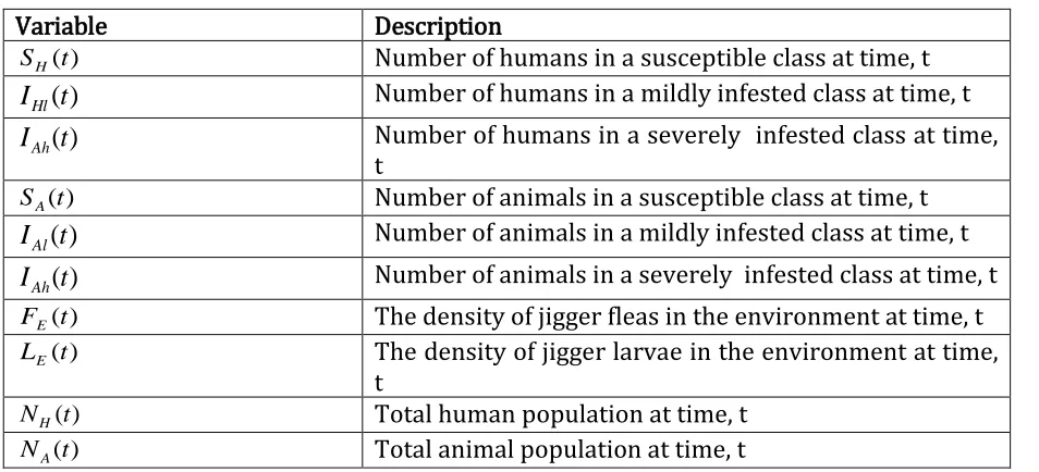
Using the above assumptions, definition of variables and parameters, the model flow diagram that depicts the dynamics of tungiasis transmission for the human population, animal reservoir population and the jigger fleas in the environment is shown in Figure 1.
Figure 1: Tungiasis basic dynamical model
Figure 1 shows the possible interactions between humans, animal reservoirs and jigger fleas in the environment. We have the susceptible humanSH, infested humans at mildly and severe statesIHl andIHh, susceptible animalSA, infested animals at mildly and severe statesIAl andIAh. We have larval class LE and the adult jigger flea classFE.
2.3Model differential equations
(1) 1 population flea Jigger in Dynamics population animal in Dynamics population human in Dynamics E E F E F Ah A E L E E L L Ah Hh E e E Ah A A Al E E F EA EA A E E F EA EA Ah Al A Al E E F EA EA A A Ah A Al A A A E E F EA EA A Ah A A A A Hh H H H E E F EH EH Hl E E F EH EH Hh Hl H Hl E E F EH EH H H Ah AH Hl H H H E E F EH EH H Ah AH H H H F k F r F I L dt dF L I I K L dt dL I I F k F r S F k F r dt dI I I F k F r S N I dt dI S S F k F r N I N b dt dS I S F k F r I F k F r dt dI I I F k F r S N I dt dI S S F k F r N I N b dt dS 1 0 and 1 0 , 1 , , , , ), ( ) ( ) ( ) ( ), ( ) ( ) ( ) ( where EA EH EA EH A Ah A AA E E F EA EA EA H Ah AH AH E E F EH EH EH Ah Al A A Hh Hl H H N I F k F r N I F k F r t I t I t S t N t I t I t S t N with initial conditions
0 ) 0 ( , 0 ) 0 ( , 0 ) 0 ( , 0 ) 0 ( , 0 ) 0 ( , 0 ) 0 ( , 0 ) 0 ( , 0 ) 0
( Hl Hh A Al Ah E E
H I I S I I L F
S
3 Properties of the model 3.1Invariant region
: matrix 8 by 8 the is ) ( (3) , , , , , , , , where (2) ) ( X A F L I I S I I S X F X X A dt dX T E E Ah Al A Hh Hl H (4) 0 0 0 0 0 0 0 0 0 0 0 0 0 0 0 0 0 0 0 0 0 0 0 0 0 0 0 0 0 0 0 0 0 0 0 0 0 0 0 0 0 0 0 0 0 0 ) ( 8 7 6 5 4 3 2 1 D D D A A D A D D A A D A D X A L A e e f e d c b a
A A
E E F EA EA e E E F EH EH b E E F EH EH c A Ah A d H Ah EH a E F F L L Ah Hh e E E F EA EA f A E E F EA EA A E E F EA EA A Ah A H H H E E F EH EH H E E F EH EH H Ah AH D F k F r A F k F r A F k F r A N I A N I A F k r D I I K D F k F r A F k F r D F k F r N I D D F k F r D F k F r N I D 6 8 7 5 4 3 2 1 , , , , , , , , , , , , , whereand F is the column vector such that:
,0,0, ,0,0,0,0
0 (5) T
A A H
HN b N
b F
)
(X
A is a Metzler matrix for all 8
X considering the fact that F0, model system (1) is positively invariant in 8
, and Fis Lipschitz continuous. Thus the feasible region for the model system is the set
(6) , , , , , , , , , : , , , , , , , 8 K F K L N I I S N I I S N I N I N S N I N I N S F L I I S I I S F L E E A Ah Al A H Hh Hl H A Ah H Al A A H Hh H Hl H H E E Ah Al A Hh Hl H
3.2Positivity of the solution
Let the initial data be
SH(t),IHl(t),IHh(t),SA(t),IAl(t),IAh(t),LE(t),FE(t)
0
then the solution set
SH(t),IHl(t),IHh(t),SA(t),IAl(t),IAh(t),LE(t),FE(t)
of the model system (1) isnon-negative for all t 0
From the first equation of the model system (1) we have
(7)
H H E E F EH EH H Ah AH H
H H H E E F EH EH H Ah AH H
H H
S F
k F r N
I dt
dS
S S
F k
F r N
I N
b dt dS
Integrating equation (7) by separating the variables we have;
t HE E F EH EH H Ah AH t
H
H ds
F k
F r N
I S
dS
0
0
0 )
0 ( )
( 0
t H
E E F EH EH H Ah
AH ds
F k
F r N
I
H H t S e
S
By using the similar procedure, it can be shown that the remaining variables E
E Ah Al A Hh
Hl I S I I L F
I , , , , , , are also non-negative for all time t0. Thus the solution set
SH(t),IHl(t),IHh(t),SA(t),IAl(t),IAh(t),LE(t),FE(t)
of the model system (1) is
non-negative for allt0.
4 Model analysis
4.1Existence of disease free equilibrium point
The disease free equilibrium (DFE) point of the model system (1) is given by
0
, 0 , 0 , 0 , ,
0 , 0 , )
, , , , , , , (
o
A A A
H H H o
E o E o Ah o Al o A o Hh o Hl o H
N b N
b F
L I I S I I S
where by NHand NAare constants with estimated values of 1500 humans and 1200 animal reservoirs respectively.
4.2Local stability of the disease free equilibrium
point has a negative trace and a positive determinant or has negative eigenvalues (Mpeshe et al., 2009). We prove the following Theorem
Theorem 1: The disease free equilibrium
o whenever it exists is locallyasymptotically stable if Ro 1and unstable otherwise.
Proof
At disease free equilibrium point o we obtain the Jacobian matrix as given in (8) as
(8)0 0 0 0 0 0 0 0 0 0 0 0 0 0 0 0 0 0 0 0 0 0 0 0 0 0 0 0 0 0 0 0 0 0 0 0 0 0 0 0 0 0 0 0 12 7 11 6 5 10 4 9 1 3 8 2 o J J J J J J J J J J J J J L A e e A A H H
, , , , , , , where 12 11 10 9 8 7 6 5 4 3 2 1 k r J k b N r J J k b N r J J J J b J J b J J J F F A A A F EA EA H H H F EH EH L L A A A A A H H AH H H The trace of
oJ is negative and its determinant is positive. Therefore all its eigenvalues have negative real parts.
J o
0Tr which in this case implies
(9) 0 3 3 k rF F L L A A H
H
J o
0Det which in this case implies
1
0 (10)1 H H A A EA EA A A A H H EH EH L F e o F H A A A L L H H H H A b N b N r R r k
k
where
F F F A A A A A A EA EA o r k r b N R
We let;
H H A A EA EA A A A H H EH EH L F e
o F
H A A A L L H H H
b N b
N r
R r
k
1
For the determinant of the Jacobian matrix
oJ to be positive must be greater than, that is and the basic reproduction number Romust be less than one
Ro1
. It follows that the condition Det
J
o
0 implies thatTr
J
o
0. Therefore, the disease free equilibrium
o is locally asymptotically stable if and only if1
o
R and thus we have
proved Theorem 1.
4.3Global stability of the disease free equilibrium
The global stability of the disease free equilibrium is determined using Metzler matrix stability method by Castillo-Chavez et al. (2002) whereby the system is put in the form:
(12)
(11)
2
1 ,
i i
i n
DFE n
o n
X B dt dX
X B X
X B dt dX
where Xn and Xi are vectors for non-transmitting and transmitting classes respectively,XDFE,n is a disease free equilibrium, and Bo,B1andB2 are matrices. For global
stability of the disease free equilibrium to hold the matrix Boshould have the eigenvalues
with negative real parts and matrix B2need to be a Metzler matrix (i.e. the off-diagonal
elements of B2 are non-negative, denoted by B2(X)0,i j).
From model system (1) we consider the following sub-systems
(13) 0
, ,
, , , , , ,
, ,
,
T
A A A H
H H n DFE
T E Ah Al Hh Hl i T E A H n
N b N b X
F I I I I X L S S X
We consider the system (11) and differentiate it with respect to SH,SAand LE at disease free equilibrium point o
(14)0 0
0 0
0 0
L L A
H o
B
Differentiating system (11) with respect to IHl,IHh,IAl,IAh,FE we obtain matrixB1in (15)
(15)
0 0
0
0 0 0
0 0 0
1
e e
A A A F EA EA A
A A
H H H F EH EH H
H AH
k N b r b
k
N b r b
B
Again from system (12) we differentiate it with respect to IHl,IHh,IAl,IAh,FE we have matrixB2as indicated in equation (16)
(16)
0 0
0
0 0
0
0 0
0
0 0
0
0 0
0
2
k r k
N b r b
k
N b r b
B
F F A
A A A F EA EA A
A A
A A A
H H H F EH EH H
H
H H AH H
We have investigated that the eigenvalues of matrix Bo are real and negative and the matrixB2 is a Metzler matrix therefore the model system (1) is globally asymptotically
stable which is supported by the following theorem.
Theorem 2: The disease-free equilibrium point
o is globally asymptotically stable ifRo1 and unstable if Ro 1
4.4Existence of endemic equilibrium points
Endemic equilibrium point * is a steady state solution in which the disease persists in the
population i.e.IHl 0,IHh 0,IAl 0,IAh 0andFE 0. We equate all expressions for the
equations in the model system (1) to zero and let *
* * * * * * * *
, , , , , ,
, Hl Hh A Al Ah E E
H I I S I I L F
S
and
*
* *
E E
F F k F
r
P considering that the animal population is constant for bA A then from model system (1) at arbitrary equilibrium solution *
(20)(19) (18) (17) * * 2 * * 2 * * * * * H A EH EH A A A A AH H EH EH H H H A A A EH Hl H EH EH A A A A AH H H A H A A A A Ah E E F P b N P N N b b N I P b N N b S b N I F k F r P
H A A A AH H H H A A A A AH H H A A A EH EH H e H H H H A A A EH EH A H e E H A EA EA A A A A A A EA EA A A A A A A A Al H A EA EA A A A A A A A A A H A EH EH A A A A AH H EH EH H H H H EH EH H A A A A EH H H EH EH Hh b N N b b N b N KN U N b b N KN D T RP QP M UP DP L P b P b b N I P b N N b S P b N P N P N b N N b P I 2 ) )( ( ) )( ( where (24) (23) ) ( (22) (21) 2 2 * 2 * * 2 * * * * * * 2 * * * * 2 * *
( ) ( )
2 ) )( ( ) ( ) ( 2 ) )( ( 2 2 L L A A A H e H A A A A AH H H H A A A A H e H A A A A AH L L H H A H H H H H A A A A A A AH e EH EH H L L A A A e H H H H e A H EH EH A A A AH H H H A A A H e H A A A AH H H H A A A A AH H H A A A EH EH H e b N b N N T b N b N N b b N b N N R b N N b N Q b N b N KN M b N N b b N b N KN U Substituting *
P and *
Ah
I from equations (17) and (18) respectively into equation (25) to solve for *
E
(26)1 (25) 0 * * * * * * * * P b N L F F k F r F I L A A A A A E L A F A E E E F E F Ah A E L
Substituting *
E
F from equation (26) into equation (17) we have
* (27)* * * * P b N L k P r b N r L r P A A A A A E L A F A F A A A A A F E F L A
F L A F A A A A A F A A A A A F A E L A F A F E F L A A E L A r C r b N k B b N r A BP P A L C P P r A r L r P AP P L BP , , where (28) * 2 * * * * * 2 * * * * *Substituting *
E
L from equation (24) into (28) we have
* 02 * 3 * 4 * * 2 * * 2 * * 2 * * * 2 * * 2 * * 2 * * AT CM P BT M CU AR P U BR CD T AQ P BQ D R QP T RP QP BP P A M UP DP C P BP P A T RP QP M UP DP C P L A L A A L A A A A L A A L A
On simplification we have the four degree polynomial function in terms of P* given by
where (29) 0 4 3 2 1 0 4 * 3 2 * 2 3 * 1 4 * 0 AT CM a BT M CU AR a U BR CD T AQ a BQ D R a Q a a P a P a P a P a L A L A A L A A A Substituting *
P from equation (17) into (29) we have the expression for the endemic equilibria which satisfy the following four degree polynomial in terms of *
E
4 3 4
3 4 3
3
2 4 2 3 2 2 2
4 3
2 2 3 1 1
4 3 2 2 3 1 4 0 0
4 * 3 2 * 2 3 * 1 4 * 0
4
6 3
4 3
2
where
(30) 0
k a Y
k a r a Y
k a k r a r a Y
k a r a r a r a Y
a r a r a r a r a Y
Y F Y F Y F Y F Y
F
F F
F F
F
F F F F
E E
E E
Since the variables * * * * * * *
, , , , ,
, Hl Hh A Al E E
H I I S I L F
S are expressed in terms of *
P then we
substitute * *
*
E E
FF k F
r
P in equation (29) we obtain the polynomial function with
degree four in (30) which represents the presence of endemic equilibrium points. This shows that there are possible four roots for *
E
F which further implies that there are at most four possible endemic equilibrium points.
4.5Global stability of endemic equilibrium point
Global stability of the endemic equilibrium (EE) is investigated using Lyapunov method and LaSalle's invariance principle. The approach which has been found to be useful for compartmental epidemic models with any number of compartments (Korobeinikov and Maini, 2004). To achieve this we construct a suitable Lyapunov function of the form:
ln
(31)8
1
*
i
i i i
i x x x
A L
where Ai is a properly selected constant, xi is the population of th
i compartment, *
i
x is the equilibrium value of xi and Ai 0. The Lyapunov function denoted by L is continuous and differentiable. We have:
(32)
ln ln
ln ln
ln ln
ln ln
, , , , , , ,
* 8
* 7
* 6
* 5
* 4
* 3
* 2
* 1
E E E E
E E
Ah Ah Ah Al
Al Al
A A A Hh
Hh Hh
Hl Hl Hl H
H H E
E Ah Al A Hh Hl H
F F F A L L L A
I I I A I I I A
S S S A I I I A
I I I A S S S A F L I I S I I S L
The global stability of endemic equilibrium (EE) holds if its time derivative 0 dt dL
. Proof:
1 1 1 1 1 1 1 1 * 8 * 7 * 6 * 5 * 4 * 3 * 2 * 1 dt dF F F A dt dL L L A dt dI I I A dt dI I I A dt dS S S A dt dI I I A dt dI I I A dt dS S S A dt dL E E E E E E Ah Ah Ah Al Al Al A A A Hl Hl Hh H H Hl H H H
EE F E E E E E E E F E E E Ah E Ah E Ah E E e E Hh E Hh E Hh E E e E L L E E Ah A A Ah Ah F EA EA E Al E E Al E E Al E Al Al Al A Al Al A F EA EA E E E A E E A E A A A A A Ah A Ah A Ah A A A A A A Hh H H Hh Hh F EH EH E Hl E E Hl E E Hl E Hl Hl Hl H Hl Hl H F EH EH E E E H E E H E H H H AH H Ah H Ah H Ah H H H H H H F k F r F k F F k F F F A F F F A L I L I L I L L K A L I L I L I L L K A L L L A I I I A r F k I F F k I F F k I F I I A I I I A S r F k F F k S F F k S F S S A S N I S I S I S S A S S S A I I I A r F k I F F k I F F k I F I I A I I I A S r F k F F k S F F k S F S S A S N I S I S I S S A S S S A dt dL 1 1 1 1 1 1 1 1 1 1 1 1 (33) 1 1 1 1 1 1 1 1 1 1 1 1 1 1 * * * 8 2 * 8 * * * 7 * * * 7 2 * 7 2 * 6 * * * * 5 2 * 5 * * * * 4 * * * 4 2 * 4 2 * 3 * * * * 2 2 * 2 * * * * 1 * * * 1 2 * 1
Z F F F A L L L A I I I A I I I A S S S A I I I A I I I A S S S A dt dL E F E E E L L E E Ah A A Ah Ah Al A Al Al A A A A Hh H H Hh Hh Hl H Hl Hl H H H H 2 * 8 2 * 7 2 * 6 2 * 5 2 * 4 2 * 3 2 * 2 2 * 1 1 1 (34) 1 1 1 1 1 1
1 01 0 1 1 1 1 0 1 1 (35) 0 1 1 0 1 1 0 1 1 0 1 1 0 1 1 ) ( where * * * 8 * * * 7 * * * 7 * * * * 5 * * * * 4 * * * 4 * * * * 2 * * * * 1 * * * 1 E E F E E E E E E E Ah e E Ah E Ah E E E Hh e E Hh E Hh E E Al F EA EA E E E Al E E Al E Al Al A F EA EA E E E A E E A E A A A A A Ah A Ah A Ah A A Hl F EH EH E E E Hl E E Hl E Hl Hl H F EH EH E E E H E E H E H H H AH H Ah H Ah H Ah H H F k F r F k F F k F F F A L I K L I L I L L A L I K L I L I L L A I r F k F F k I F F k I F I I A S r F k F F k S F F k S F S S A S N I S I S I S S A I r F k F F k I F F k I F I I A S r F k F F k S F F k S F S S A S N I S I S I S S A Z ) (
is non-positive by following the approach of Korobeinikov (2002, 2004, 2007) and McCluskey (2006). Thus ()0 for all 0 Hence, 0
dt dL
in and is zero
when*. Therefore the largest invariant set in such that
0
dt dL
is the singleton
) (*
Theorem 5: The endemic equilibrium point * of model system (3) is globally asymptotically stable in if Ro 1 and unstable otherwise.
5 Simulations on the basic model state variables over time
The simulation of the model is conducted to find out the dynamics of Tungiasis disease in the population when there is no intervention. It is performed using MALAB, and we set time in weeks and days. We use parameter values whose sources are from literature and others are estimated. Furthermore through numerical simulation we illustrate the stability of the endemic equilibrium states in human, animal reservoirs and flea in the environment whenever they exist. The parameter values used for simulation are shown in Table 3.
5.1Parameter Estimation
In this section we estimate some of the parameter values of Tungiasis model. We estimate the human mortality rateH, taking into consideration that the average life expectancy of the human population in Tanzania is 60.9 years (UNICEF, 2015) which is equivalently to
5 10 5 .
4 per day. According to Tanzania population (TP, 2016) the human birth rate is 0.00011 per day. The maturation rate L of larvae into adult flea is estimated to be 0.0105 per day and the shedding rate of fleas A to be 0.4 per day. The death of the flea occurs around day 25 post-penetration (Eisele et al., 2003), we therefore assume the life span of a flea to be 25 days, which implies that its death rate F is 0.04 per day. The concentration of jigger fleas in the soil environment is not known; we therefore consider the number of fleas in one cubic meter of sand and assume the maximal larvae carrying capacity K to be
3 5
m / cell 10
1 and the half saturation constant for fleas k to be 4 3
m / cell 10
1 . The disease
induced death rate for animal reservoir population A is estimated to be 0.037 per day and the disease induced death rate for human population H is estimated to be 0.011 per day. The natural death rate of animal reservoir A ranges from
3603600
days(Radostits, 2001; Gaff et al., 2007). The values of effective contact rates are A0.26 per day (Allerson et al., 2013), AH 0.052 per day (Gaff et al., 2007), EH 0.19per day andday per 48 . 0
EA
Table 3: Parameter values used for the simulation of model variables
Parameter Value/Range Source/References
k 4 3
m / cell 10
1 Estimated
K 5 3
m / cell 10
1 Estimated
L
0.0105per day Estimated
H
0.011 per day Estimated
A
0.037 per day Estimated
H
0.000045 per day UNICEF. (2015)
A
13600 360
0028 .
0 per
day
Gaff et al. (2007); Radostits. (2001)
F
0.04 per day Eisele et al. (2003),
F
r 0.58 per day Estimated
L
0.08 per day Estimated
EH
0.19 per day Estimated
EA
0.48 per day Estimated
AH
0.052 per day Gaff et al. (2007)
A
0.26 (0.091-0.9) per day Allerson et al. (2013)
H
b 0.00011 per day TP, (2016).
A
b 0.022 per day Gaff et al. (2007)
A
0.40 per day Estimated
e
0.12 per day Estimated
EH
0.4 Estimated
EA
5.2Discussion of the results
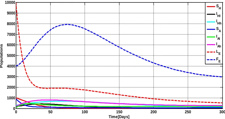
Figure 2 illustrate the dynamics in humans, animal reservoirs and flea populations, showing the behavior of eight state variables SH,IHl,IHh,SA,IAl,IAh,LE and FE over time when there is no intervention.
0 50 100 150 200 250 300
0 1000 2000 3000 4000 5000 6000 7000 8000 9000 10000
Time[Days]
Pop
ula
tion
s
S
H
I
Hl
I
Hh
S
A
I
Al
I
Ah
L
E
F
E
Figure 2: Dynamics in model sub-populations
from the flea infested environment. The decrease of susceptible animal reservoirs results into the growth of the mildly infested animal reservoirs that grow exponentially and then start declining due to natural death and as the acquire more infestation from the environment to join severely infested animal reservoirs class then eventually attain endemic equilibrium point. The severely infested animal reservoirs grow exponentially to a certain point in time then start declining due to natural and disease induced mortalities and finally they attain endemic equilibrium point.
5.3The variation of population variables on the dynamics of Tungiasis over time
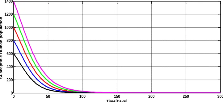
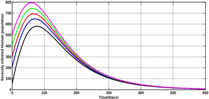
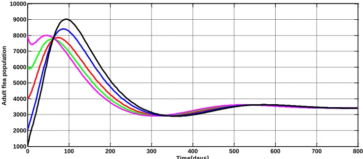
The numerical simulations as illustrated in Figures 3(a), 3(b), 3(c), 4(a), 4(b), 4(c), 5(a) and 5(b) show the variations of the model variables SH,IHl,IHh,SA,IAl,IAh,LEandFE over time. The trajectories of the model variables originating from different initial values converges to a common endemic equilibrium levels which implies the existence and stability of the endemic equilibrium states in human, animal reservoirs and flea populations whenever they exist.
0 50 100 150 200 250 300
0 200 400 600 800 1000 1200 1400
Time[Days]
Sus
cep
tible
Hum
an
pop
ula
tion
Figure 3(a): Stability of the endemic equilibrium for susceptible human population
0 50 100 150 200 250 300
0 100 200 300 400 500 600
Time[Days]
Mildily inf
ested Human populati
Figure 3(b): Stability of endemic equilibrium for mildly infested human population
0 100 200 300 400 500 600
0 100 200 300 400 500 600 700 800
Time[Days]
Se
ver
ely
infe
ste
d Hu
ma
n po
pula
tion
Figure 3(c): Stability of the endemic equilibrium for severely infested human population
0 20 40 60 80 100 120 140 160 180 200
0 500 1000 1500
Time[Days]
Sus
cep
tible
an
ima
l po
pula
tion
Figure 4(a): Stability of the endemic equilibrium for susceptible animal population
0 20 40 60 80 100 120 140 160 180
0 100 200 300 400 500 600 700 800
Time[Days]
Mildly inf
ested animal populat
ion
0 50 100 150 200 250 300 0
200 400 600 800 1000 1200
Time[Days]
Se
ver
ely
infe
ste
d a
nim
al p
opu
lati
on
Figure 4(c): Stability of the endemic equilibrium for severely infested animal population
0 50 100 150
0 0.2 0.4 0.6 0.8 1 1.2 1.4 1.6 1.8
2x 10
4
Time[days]
Jigger
Larvae pop
ulati
on
Figure 5(a): Stability of the endemic equilibrium for jigger larvae population. .
0 100 200 300 400 500 600 700 800
1000 2000 3000 4000 5000 6000 7000 8000 9000 10000
Time[days]
Adu
lt fle
a p
opu
lati
on
6 Conclusions
The Tungiasis model with sub-models of humans, animal reservoirs and flea populations, has been developed and analyzed to study the tungiasis dynamics in endemic areas. The basic reproduction numberR0 computed was used to determine the stability of the
disease-free equilibrium point (DFE). We then proved the existence and stability of endemic equilibrium point (EE) using Lyapunov direct Method combined with LaSalle’s Invariance Principle. The analytical results show that the DFE is locally asymptotically stable, if R0 1
and the EE is globally asymptotically stable whenR0 1. From numerical simulations we
have observed that without intervention the populations vary for some time but ultimately approach the endemic equilibrium levels in the long run which imply the existence and stability of endemic equilibrium point.
This work provides a basic dynamical model that can be used to understand the transmission dynamics of tungiasis transmission that involves the interaction between human population, animal reservoir population and the flea infested environment. Understanding tungiasis transmission dynamics will help to design proper control strategies and evaluate their potential impact in reducing tungiasis morbidity and mortality in the endemic communities at large.
References
[1] Allerson, M., Deen, J., Detmer, S. E., Gramer, M. R., Joo, H. S., Romagosa, A., and Torremorell, M. (2013). The impact of maternally derived immunity on influenza A virus transmission in neonatal pig populations. Vaccine, 31(3), 500-505.
[2] Bawa, M., Abdulrahman, S., Jimoh, O., and Adabara, N. (2013). Stability analysis of the disease-free equilibrium state for lassa fever disease. Journal of Science, Technology, Mathematics and Education (JOSTMED), 9(2), 115-123.
[3] Castillo-Chávez, C., Feng, Z., and Huang, W. (2002). On the computation of basic reproduction number and its role in global stability. Mathematical approaches for emerging and reemerging infectious diseases: an introduction, 1, 229.
[4] Eisele, M., Heukelbach, J., Van Marck, E., Mehlhorn, H., Meckes, O., Franck, S., and Feldmeier, H. (2003). Investigations on the biology, epidemiology, pathology and control of Tunga penetrans in Brazil: I. Natural history of tungiasis in man. Parasitology research, 90(2), 87-99.
[5] Feldmeier H, Sentongo E, Krantz I (2012) Tungiasis (sand flea disease): a parasitic disease with intriguing challenges for a transformed public health. Eur J Clin Microbiol Infect Dis 32:19-26
[6] Gaff, H. D., Hartley, D. M., and Leahy, N. P. (2007). An epidemiological model of Rift Valley fever. Electronic Journal of Differential Equations, 2007(115), 1-12.
[7] Gupta, A., Briat, C., and Khammash, M. (2014). A scalable computational framework for establishing long-term behavior of stochastic reaction networks. PLoS Comput Biol, 10(6), e1003669.
[8] Heukelbach, J., De Oliveira, F. A. S., Hesse, G., a Feldmeier, H. (2001). Tungiasis: a neglected health problem of poor communities. Tropical Medicine & International Health, 6(4), 267-272.