MODELING OF THE FUNCTION OF THE OZONE
CONCENTRATION DISTRIBUTION OF SURFACE TO URBAN
AREAS
Amaury de Souza,
[a]*Soetânia S. de Oliveira,
[b]Flavio Aristone,
[a]Zaccheus
Olaofe,
[c]Shiva Prashanth Kumar Kodicherla,
[d]Milica Arsić,
[e]Nabila
Ihaddadene
[f]and Ihaddadene Razika
[g]Keywords: Ozone distribution of probability, air monitoring, Weibull distribution.
In large urban centers, the major contributors to much of the degradation of air quality are motor vehicles on the road. In some cities, the levels of concentrations of air pollutants have reached levels that pose a risk to human health. Ozone (O3) is a secondary pollutant formed
from photochemical reactions of nitrogen oxides (NOx). Numerous studies have found associations between daily levels of ozone with a
number of health effects. In the state of South Mato Grosso (MS), there has been a growing increase of ozone levels in the atmosphere in recent years. Considering the above, this study aimed to identify the best estimator for the Weibull distribution, in analyzing the ozone
concentration, for the city of Campo Grande-MS. For this, electronic data from the continuous air monitoring station located on the campus
of the Federal University of South Mato Grosso (UFMS), Campo Grande was utilized. According to the results presented by the tests, it was verified that the LSRM method presented the poorest performance. The EPFM, MOM and MSDM are most efficient methods to adjust the Weibull distribution curves for the evaluation of ozone concentrations in the atmosphere.
*Corresponding Authors
E-Mail: [email protected]
[a] Universidade Federal de Mato Grosso do Sul, Campo Grande, MS, Brasil
[b] University of Campina Grande, PB, Brazil.
[c] University of Cape Town: Rondebosch, Western cape, South Africa
[d] Department of Civil Engineering, Room No. EB 577, Engineering Building (EB), Xi'an Jiaotong-Liverpool University (XJTLU), Suzhou Industrial Park, Suzhou, P. R. China.
[e] University of Belgrade, Technical faculty in Bor, Serbia. [f] Department of Mechanical Engineering, M'Sila University,
B.P 166 Ichbelia, M'Sila 28000, Algeria.
[g] Department of Mechanics, Mohamed Boudiaf University, M'sila, Algeria.
Introduction
Ozone (O3) and nitrogen oxides (NOx) comprising of
nitrogen dioxide (NO2) and nitric oxide (NO) are among the
most important contaminants in urban areas as they have adverse effects on human health and the natural environment. The main source of NOx in urban areas is the exhaustion of motor vehicles. The main proportion of NOx is emitted as NO, while a smaller proportion is emitted directly as NO2. Even if the concentration of NOx has a
downward trend, NO2 share in NOx emissions has increased
in recent years and depends on vehicle type fuel technology, exhaust treatment technology and the driving conditions.1
In South Mato Grosso, measurement of ozone concentration at ground level began in 2004. The ozone concentration has shown an increasing trend in the state of South Mato Grosso since the first measurements took place in 2004, and this has been the main pollutant in many areas
of the state.2-4
Since most existing policies to reduce tropospheric levels of O3 in urban areas focus on reducing precursor emissions,
their success depends heavily on an accurate development of the sensitivity of the O3 production. The European Union
(EU) has established air quality standards for ambient ozone concentrations. Directive 2008/50 defines information and alert thresholds which refer to hourly values and equal to 180 and 240 mg m-3. The same directive also defines a
guideline for the protection of human health and the maximum daily average value of 8 hours should not exceed the target value of 120 mg m-3 on more than 25 days per the
calendar year over a period of three years.
In Brazil, there is the CONAMA Resolution of July 28, 1990, which defines atmospheric pollution and establishes the pollution limits of any form of matter or energy with intensity and in quantity, concentration, time or characteristics in disagreement with the established levels,
that renders the air inappropriate, harmful or offensive to health, inconvenience to the public welfare, damage to materials useful for fauna and flora, detrimental to safety, use and enjoyment of property, and normal community activities.5
Monitoring data and scientific studies on ambient air quality show that some of the air pollutants in several major cities were increasing over time and not always at acceptable levels according to WHO standard. There are very limited sampled data and few case studies focusing on air pollution in Brazil, while most air modelling cases using probability distribution have been applied in foreign countries. Although such application is almost non-existent in Brazil, it is an attractive analytical option since it can reasonably predict the return period and its concentration in the subsequent period to meet evolving information needed for environmental quality management.
probability distributions have been used to adjust the concentrations of air pollutants which include Weibull distribution.7 lognormal distribution,8 range distribution,9
Rayleigh distribution,10 distribution of Gumbel11 and
distribution of Frechet.12 From scientific findings, Lu 13 and
Chen et al.14 studied the fit for selected probability
distributions using various performance indicators, such as the mean absolute error (MAE), root mean square error (RMSE), concordance index (d2), bias (B), absolute normalized error (NAE), prediction accuracy (BP) and determination coefficient (R2). The objective of this study is
to analyze and compare the Weibull distribution parameters in five cities with the results obtained for Campo Grande for modelling of the ozone concentration in MS, Brazil.
Experimental
Studied area and observational data
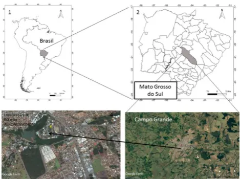
Campo Grande is the capital city of South Mato Grosso (MS) state, located in the south of Brazil Midwest region,
and sited in the centre of the state. Geographically the considered city is near to the Brazilian border with Paraguay and Bolivia. It is located at 20°26’34’’ South and 54°38’47’’ West. Figure 1 shows the location of Campo Grande in the state of South Mato Grosso.
Figure 1. Location of the Municipality of Campo Grande in the State of South Mato Grosso, and the continuous air monitoring station.
The city occupies the total area of 8,096.051 km² or 3,126 mi², representing 2.26 % of the total state area, within 860,000 inhabitants (2016) and a corresponding HDI of 0.78. The urban area is approximately 154.45 km² or 60 mi², where tropical climate and dry seasons predominate, with two clearly defined seasons: warm and humid in summer, and less rainy and mild temperatures in winter. During the months of winter, the temperature can drop considerably, arriving on certain occasions to the thermal sensation of 0ºC or 32ºF with occasional light freezing.
The yearly average precipitation is estimated at 1,534 mm, with small up or down variations. The main pollution problems in the city are attributed to the traffic of vehicles, the rise of building activities, the presence of dumping
supply electric grids power, and to the induced fire outbreak used to clean up local terrains.
The instruments used for the measurements are recorded in Table 1.
Meteorology
For the development of this work, we used electronic data from the continuous air monitoring station located on the campus of the Federal University of Mato Grosso do Sul, Campo Grande (MS), as shown in Figure 1.
Table 1. Instrumentation for measuring the atmospheric pollutants and meteorological parameters
Parameter Ozone
Instrument model Thermo Environmental 49C
Detector Chemiluminescence
PA Equivalent Method Number
EQOA-0880-047
Error (±) 1 ppb
Probability Distributions
In order to model the sampled data sets for South Mato Grosso, Weibull probability distributions were used. Performance indicators are calculated by comparing the observed values with predicted values. The observed values are the classified values of the monitoring data, while the
predicted values are the values obtained from the adjusted distribution of any statistical function.
Weibull distribution
The distribution function of Weibull two parameters for the concentration of ozone emission is expressed by the probability density function (eqn.1) where f (v) is the probability of observed ozone concentration (v), k is the dimensionless Weibull parameter/factor and c is the Weibull scale parameter (m s-1). The scale parameter can be related
to the mean ozone concentration through the shape factor, which is the consistency of ozone concentration at a given location.
𝐹(𝑣) =𝑑𝑓(𝑣) 𝑑𝑣 = (
𝑘 𝑐) (
𝑣 𝑐)
k−1
𝑒𝑥𝑝 [− (𝑣 𝑐)
k
] (1)
The cumulative distribution F(v) is an integral part of the probability density function and can be expressed eqn. (2).
𝐹(𝑣) = ∫ 𝑓(𝑣)𝑑𝑣Vv = 1 − 𝑒(𝑣𝑉) 𝑘
(2)
The entire distributions can be used to resolve the probability of occurrence affecting the shape of probability curve of the wind regime. The cumulative curve probability nature typically fits the Weibull distribution function.
Energy pattern factor method (EPFM)
The energy pattern factor is connected to the average data of ozone concentration and can be defined as the ratio of the mean of cubic ozone concentration to the cube of mean ozone concentration. The energy pattern factor (EPF) can be expressed as eqn. (3), where vi is the wind speed in meter per
second for ith observation, N is the total number of ozone
concentration observations, and 𝑣̅ is the monthly mean wind speed.
𝐸𝑃𝐹 = 1 𝑣̅3 (∑
𝑣i3
𝑁 n
i=1 ) = 𝛤(1+3
𝑘)
𝛤3(1+1 𝑘)
(3)
Once EPF is calculated, the Weibull shape and scale factors can be estimated from the following formulae.
𝑘 = 1 + 3.69
𝐸𝑃𝐹2 (4)
𝑐 = 𝑣̅
𝛤(1+1𝑘) (5)
Least-squares regression method (LSRM)
LSRM is well known as a graphical method implemented by plotting a graph in such a way that the cumulative Weibull distribution becomes a straight line where the time - series data must be sorted into bins. The equation of PDF,15
after transformation and taking into consideration of natural logarithms on both sides, the expression can be written as eqn. (6)
𝑙𝑛[− 𝑙𝑛(1 − 𝐹(𝑣))] = 𝑘. 𝑙𝑛(𝑣) − 𝑘. 𝑙𝑛(𝑐) (6)
Therefore, eqn. (6) is linear and can be fitted using the following least square regression method.
𝑦 = 𝑎𝑥 + 𝑏, 𝑦 = 𝑙 𝑛[−𝑙 𝑛(1 − 𝐹(𝑣))], 𝑥 = 𝑙 𝑛(𝑣),
𝑏 = −𝑘 ln(𝑐),𝑘 = 𝑎; 𝑐 = 𝑒−bk (7)
The cumulative distribution function, F(v) can be easily estimated from an estimator (eqn. 8), which is the median rank according to Benard’s approximation, where i is the number of the wind speed measurements and N is the total number of observations.16
The relationship between ln (𝑣) as a function of
ln (−ln (1 − 𝐹(𝑣))) represents a straight line with slope k, and the intersection point with Weibull line gives the value of scale parameter (c) derived from ozone concentration in part per billion (ppb).
𝐹(𝑣) = 𝑖−0.3
𝑁+0.4 (8)
Method of moments (MOM)
MOM is one of the iterative techniques commonly used in the field of applied sciences for evaluating the Weibull parameters. It is based on the numerical iteration of mean (𝑣̅) and standard deviations (σ) of ozone concentration and expressed as follows.
𝑣̅ =1 𝑛∑(𝑣i)
n
i=1
and 𝜎 = 𝑐 [𝛤 (1 +2 𝑘) − 𝛤
2(1 +1 𝑘)]
1 2
𝜎 𝑣̅= √
𝛤 (1+2
𝑘)
[𝛤(1+1𝑘)]2
− 1 (9)
The dimensionless Weibull and scale parameters can be calculated by eqns. (10) and (11).
𝑘 = (0.9874 𝜑 𝑣⁄ )
1.0983
(10)
𝑣̅ = 𝑐𝛤 (1 +1
𝑘) (11)
The average ozone concentration can be expressed as a function of Weibull scale parameter (c) and dimensionless Weibull shape parameter (k) derived from the Gamma function defined in eqn. (12), where 𝑦 = (𝑣/𝑐)𝑘 e(𝑣/𝑐) = 𝑦𝑥−1 𝑎𝑛𝑑 𝑥 = 1 + 1/𝑘 . Therefore, the expression is
reduced to eqn. (13).
𝛤(𝑥) = ∫ 𝑦∞ x−1 𝑒−y𝑑𝑥
0 (12)
𝑣̅ = 𝑐𝛤 (1 +1
𝑘) = 0.8525 + 0.0135𝑘 + 𝑒
−(2+3(k−1)) (13)
Mean standard deviation method (MSDM)
MSDM is used where only the two parameters such as the mean wind speed and standard deviations are available. It is well known as an empirical method and could be considered as a unique case of MOM method, in which the Weibull
shape and scale parameters are estimated by eqns. (14) and (15), where σ is the standard deviation and 𝑣̅ is the mean ozone concentration in ppb. Alternatively, Weibull scale parameter can be projected from the following expression given by eqn. (16).
𝑘 = (𝜎 𝑣)
1.086
(14)
𝑐 = 𝑣̅
𝛤(1+1𝑘) (15)
𝑐 = 𝑣̅ 𝑘2.6674
Statistical Accuracy Analysis / Goodness of Fit
To find the best model method for analysis, several statistical tools have been used by researchers to analyze the efficiency of above-mentioned methods. The following tests are utilized as follows:
(a) Relative percentage error (RPE)
𝑅𝑃𝐸 (%) = (𝑥i,w−𝑦i,m
𝑦i,m ) × 100 (17)
(b) Root mean square error (RMSE)
𝑅𝑀𝑆𝐸 = [1
𝑁 ∑ (𝑥i,w− 𝑦i,m) 2 n
i=1 ]
1 2
(18)
(c) Mean percentage error (MPE)
𝑀𝑃𝐸 = 1 𝑁 ∑ (
𝑥i,w−𝑦i,m
𝑦i,m ) ∗ 100% n
i=1 (19)
(d) Mean absolute percentage error (MAPE)
𝑀𝐴𝑃𝐸 =1 𝑁 ∑ |
𝑥i,w−𝑦i,m
𝑦i,m | ∗ 100%
n
i=1 (20)
(e) Chi square error
𝜒2=∑ni=1(𝑥i,w−𝑦i,m)2
𝑦i,m (21)
(f) Kolmogorov – Smirnov test
𝑄95= 1.36
√𝑁 (22)
(g) Analysis of variance (or) Regression coefficient
𝑅2=∑ (𝑦i,m−𝑧i,v̅) 2
−∑Ni=1(𝑦i,m−𝑥i,w)2
N i=1
∑Ni=1(𝑦i,m−𝑧i,v̅)2
(23)
where
N is the number of ozone concentration observations,
yi,m is the frequency of observation of ith calculated
value from measured data,
xiw is the frequency of ith calculated value from the
Weibull distribution and
zi,v is the mean of ith calculated value from the
measured dataset.
In general, RPE shows the percentage deviation between the calculated values from the Weibull distribution and the calculated values from measured data. Similarly, the MPE
calculated values of the Weibull distribution and the calculated values from measured data, and MAPE shows the absolute average of percentage deviation between the calculated values of the Weibull distribution and the calculated values from measured data. Perfect results are obtained when these values are nearest to zero. Regression coefficient (R2)determines the linear relationship between the calculated values from the Weibull distribution and measured data. An ideal value of regression coefficient is equal to 1.
Coefficient of Variation (COV)
COV is defined as the ratio between the mean standard deviation to the mean ozone concentration expressed in terms of percentage. It demonstrates the uncertainty of ozone concentration and can be expressed as eqn. (24), where σ is the standard deviation and v is the mean wind speed (m s-1).
𝐶𝑂𝑉(%) =𝜎
𝑣̅× 100 (24)
RESULTS AND DISCUSSION
The description of statistics of ozone concentration for the sampling period of 2015 is shown in Table 2. The mean value of the ozone concentration was higher than the median indicating that there was a high concentration recorded during the study period, the positive numbers indicate roughness effect that defines the occurrence of extreme events and the emissions of ozone gas.
Table 2. Descriptive analysis of ozone concentration for the sampling period (2015)
Months Jan Feb Mar Apr May Jun Jul Aug Sep Oct Nov Dec
Mean 21.60 16.46 16.75 16.70 13.23 11.28 12.41 17.01 18.88 16.94 16.11 15.97
StDev 11.45 9.09 9.36 9.73 7.06 7.69 8.04 13.20 11.06 8.83 7.75 7.61
Cvariation 53.00 55.26 55.89 58.27 53.38 68.15 64.76 77.60 58.57 52.13 48.10 47.66
Median 18.90 15.25 15.80 15.50 13.20 10.20 12.10 15.55 17.60 15.80 15.20 14.75
Minimum 1.90 2.20 2.20 2.10 2.00 2.00 2.00 1.60 2.00 2.00 2.30 1.00
Maximum 79.7 70.9 58.5 61.2 41.3 34.5 44.4 55.9 57.7 47.7 46.6 36.4
Skewness 1.13 1.39 0.96 1.11 0.40 0.38 0.47 0.65 0.71 0.71 0.67 0.42
Kurtosis 2.11 4.98 1.49 1.95 0.11 -1.04 -0.32 -0.44 0.38 0.47 0.44 -0.54
Count 742 672 742 742 742 720 742 742 720 742 720 742
k 1.99 4.98 1.88 1.80 1.99 1.52 1.59 1.31 1.78 2.03 2.21 2.23
O3 (ppb) 24.36 17.93 18.81 18.76 15.03 12.51 13.71 18.43 21.13 19.11 18.19 18.00
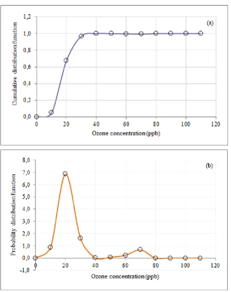
These results also show how ozone distributions were distorted to the right. Most of the sampled data was concentrated to the left of the PDF chart (Figure 3b) with few high values of ozone concentration (ppb). An average, a median, roughness and persuasion values have increased, indicating a growing problem of air pollution in Campo Grande.
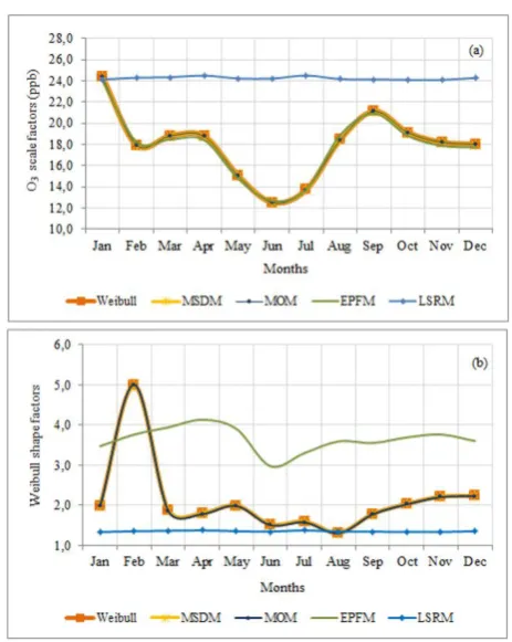
Figure 2 shows the plots of monthly variations of the Weibull distributions generated by four statistical approaches considered for the Weibull shape and scale parameters. It can be seen that the divergence of the parameters of the form and the methods is more significant than the parameters of the scale. The dimensionless Weibull shape parameters observed less significant values obtained from EPFM and LSRM. Consistency is achieved in the Weibull scale parameters, and both MOM and MSDM have a comparable range of Weibull scale and shape parameters.
Table 2 lists the expressive ozone concentration statistics, which show evident variations for different time periods. The range of the ozone concentration can be represented as the discrepancy between the maximum and minimum ozone concentration. The concentration of ozone varies between 1 and 79.7 ppb with a mean value of 16.1 ppb. Likewise, standard deviations range from 13.2 to 7.06 ppb.
The critical values at 95 % confidence level in the Kolmogorov-Smirnov (Q95) test are 0.0248 and 0.0246 for months at 31 days and 30 days, respectively. In the end, the maximum error in the CDF never exceeds the corresponding significant values, which implies that the proposed technique is applicable to generate the necessary variables in the selection of the site.
Figure 3 shows the histogram and the comparison of the Weibull probability functions of the monthly average ozone concentration. The ozone data robustly characterized by the Weibull probability density function (PDF) and the cumulative distribution function (CDF). The maximum CDF errors are below or close to critical values in the Kolmogorov-Smirnov test at the 95 % confidence level. A similar behaviour was observed and the least squares regression method does not satisfy precisely all other methods.
Figure 3. CDF (a) and PDF (b) plots for Weibull distribution obtained for 2015.
It is observed that for the Weibull distribution, the parameter of form k oscillated considerably in the comparison between the months, varying from 4.9815 to 1.3137, with the lowest value occurring in August and the highest value in the month of February, it is observed that the value of k is inversely related to the variance of the ozone concentration, which implies low variances if k is high and vice versa. In this sense, the values of k obtained for Campo Grande were in full agreement with the previous statement, where the highest values of k were related to the smallest variances shown in Table 2. The scale parameter c
In order to compare the quality of the PDFs to sample variable concentration data, several statistics were used in related studies for O3 analysis. The most used are the
coefficient of determination, the results of the Chi-square test (χ2), and the mean square error (RMSE). In most studies,
a visual evaluation of the adjusted PDFs superimposed on the data histograms is also performed. The RMSE is applied in theoretical cumulative probabilities against empirical or theoretical cumulative probabilities of the concentrations of the observed variables. These statistics are also calculated with variable data in the form of frequency histograms.
In addition to the analysis performed on the variable distributions, some authors also evaluated the adequacy of PDFs to adjust the concentration distributions obtained by the sample variables or to predict the concentrations. In this case, the PDFs are first adjusted to the variables data. Then, the theoretical density distributions are derived from the PDFs adjusted for the variables. Finally, the fit quality measures are calculated using the theoretical density distributions and the distribution estimated from the O3
variables of the sample.
The performance of these PDFs to evaluate the concentrations of the variables was also analyzed and the results are summarized in Table 2. It can be said that the evaluation of these distribution functions based on the quality of the adjustment criteria alone is not enough. These criteria should be used to identify appropriate distributions before a detailed analysis is done. Because these installed PDFs can be used for different applications by industries, public decision-makers, the performance of these PDFs for specific applications, such as the predicted concentration of pollutants, should also be evaluated. The results show that there are underestimation and overestimation of the concentration density of the pollutant in general, depending on the concentration range. The percentage errors show mainly that this underestimation and overestimation of the concentrations of these pollutants, which may be due to the effect of heating and the atmosphere.
The concentration of ozone increases slowly after sunrise, peaking during the day and then decreasing until the following morning. This is due to the photochemical formation of O3. The shape and amplitude of ozone cycles
are strongly influenced by climatic conditions (solar radiation) and by prevailing levels of precursors (NOx).
For example, Hsieh and Liao17 argued that the probability
distributions for all air pollutants in Taiwan were approximate to be a lognormal distribution. Besides that, Neustadter et al18 revealed that the total suspended
particulate is obviously logically distributed, whereas sulfur dioxide and nitrogen dioxide are rationally estimated by lognormal distributions. However, Oguntunde et al19 showed
that the Gamma distribution is the best distribution for carbon monoxide concentration modelling in Lagos State, Nigeria. Kan and Chen20 indicated that the best fit
distributions for PM10 concentrations in Shanghai were lognormal.
In Malaysia, Noor et al21 found that the best distribution
fits of the PM10 observations in Nilai was the Gamma distribution while the log-normal distribution is more appropriate in Shah Alam. Razali et al22 refer to the
to carbon monoxide data in Bangi, Malaysia. Consequently, there is no common distribution of air pollutants and it differs by region and time studied. It is important to conduct a comparative analysis to find out which distribution best fits the air pollutants at a specific location in order to provide a better estimate of the air quality at that location.
The four methods mentioned above were used to estimate the two Weibull parameters, i.e., shape and scale parameters. These values are averaged and presented in Figures 2a and 2b It can be clearly seen that a strong linear relationship between the monthly parameters of the Weibull average scale and the mean concentration measure of ozone. The values of the regression coefficients (R2) are extremely high
and show a counterpart to the linear model (R2 = 0.999927).
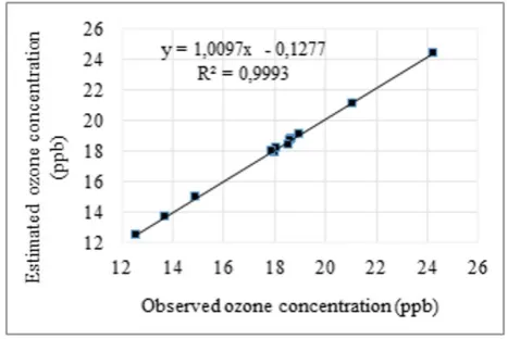
Figure 4 shows the linear relationship between the Weibull scale parameter and the monthly mean values observed in Campo Grande, the correlation between the monthly scale parameter, and the monthly average ozone concentration measured, a linear relationship was found with a directly proportional slope to the average of the monthly parameters of the scale k.
Figure 4. The relation between Weibull O3 parameters monthly
scaled (averages of all four methods) and the mean values of the average ozone concentration.
The ozone concentration can be demonstrated by the coefficient of variation. It can be defined as the ratio between the standard deviation of the ozone concentration and is an indicator and not an absolute value. The average monthly VOC values are shown in Table 2. The coefficient of variation varies from 77.60 to 47.65 % and the highest percentage variation in the month of August. In general, the VOC is lower when the concentration of ozone is maximum and vice versa.
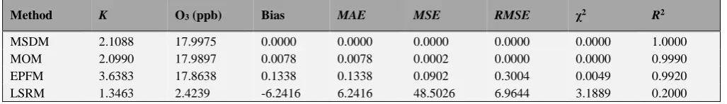
To judge the relative efficiency of the statistical methods, six statistical tools, i.e., RPE, RMSE, MPE, MAPE, χ2 and R2 are employed. Many researchers have already used
methods at different geographic locations to estimate ozone concentration. In general, only one column is needed to classify statistical methods, since the above approaches give virtually identical results. For a more accurate diagnosis, these six statistical tools were used to classify the methods.
Table 5. Relative efficiency of statistical methods used.
Method K O3 (ppb) Bias MAE MSE RMSE χ2 R2
MSDM 2.1088 17.9975 0.0000 0.0000 0.0000 0.0000 0.0000 1.0000
MOM 2.0990 17.9897 0.0078 0.0078 0.0002 0.0000 0.0000 0.9990
EPFM 3.6383 17.8638 0.1338 0.1338 0.0902 0.3004 0.0049 0.9920
LSRM 1.3463 2.4239 -6.2416 6.2416 48.5026 6.9644 3.1889 0.2000
The average monthly variation of the amplitude observed in the ozone concentration (10.32 ppb) can be attributed to the fact that it is related to the winter solstice. At this time, the region under study suffers from the constant penetration of cold fronts coming from the South, these cold fronts alter the fields of atmospheric pressure and can directly influence the direction and speed of the wind. The north-east, northwest-northeast, west, east and north-northwest winds occur every month of the year. In these directions, the northwest direction is what predominates more in the region.
With the entry of cold front, there is a decrease in pressure, causing the wind to recede and increase its speed. During its passage, there is an increase in atmospheric pressure, causing sudden changes in the direction of the wind, which is usually accompanied by bursts. As with the front, the pressure rises slowly and continuously and can present bursts with subsequent stability.23
It is known that the climate of the region and the entire state is influenced by several factors, such as the infiltration of cold air masses, especially during the winter months, possibly the Atlantic Polar Mass. Another mechanism that has been changing the region's climate in recent years is the "El Niño" and "La Niña" phenomena.24
With respect to the Atlantic Polar Mass, with continental dislocation, it originates on the sub-Antarctic waters to the south of South America, penetrates in the state by West and Southwest and predominates in autumn and winter. It is dry and does not get moisture throughout the season. The Atlantic Polar Mass with maritime displacement also originates to the south of the South American continent, predominates during the winter and the spring. It is dry at the source and absorbs moisture from the ocean, mainly from the warm current of Brazil.25
These results prove the need to carry out regional studies by testing a greater number of probabilistic models for the adjustment of this climatic variable, since physical space peculiarities and the interference of climatic phenomena in the region, in monthly, daily and even hourly, are able to change the behavior of the ozone-climate variable significantly. As shown in Tables 3 and 4 discussed above, the Weibull distribution adequately adjusted the mean wind concentration data. This extremely important result could only be verified by the investigation of a probabilistic model less used in other studies and regions.
CONCLUSIONS
Parameter estimation is one of the important steps in assembling distribution, allowing predictions to be made accurately. The objective of this study was to compare several parameter estimators and to find the most appropriate estimator and distribution to predict ozone concentration. The quality and reliability of the models developed were evaluated through four performance indicators and the result of this study shows that the EPFM, MOM and MSDM is the most appropriate method to estimate the parameter for Campo Grande using the Weibull distribution.
From the analysis of the test results, it was evidently revealed that LSRM presented worse performance than other methods. The EPFM, MOM and MSDM methods are the most efficient methods to adjust the Weibull distribution curves for the evaluation of ozone concentration data.
The study revealed that the air quality status was not good at all times. Four distributions were compared and the Weibull distribution offers the best fit because three performance indicators offer the best results for this distribution. The scatter plot of observed O3 concentrations
versus predicted values obtained from the Weibull distribution shows a very good fit with the coefficient of determination of 0.999.
REFERENCES
1Carslaw, D. C., Evidence of an increasing NO2/NOX emissions
ratio from road traffic emissions, Atmos. Environ., 2005,
39(26), 4793-4802. DOI:
https://doi.org/10.1016/j.atmosenv.2005.06.023
2Souza, A., Aristone, F., Kumar, U., Kovač-Andrić, Arsić, M.,
Ikefuti, Sabbah, I., Analysis of the correlations between NO, NO2 and O3 concentrations in Campo Grande – MS, Brazil,
Eur. Chem. Bull., 2017, 6(7), 284-291.
DOI: http://dx.doi.org/10.17628/ecb.2017.6.284-291
3Souza, A., Fernandes, W. A., Surface ozone measurements and
meteorological influences in the urban atmosphere of Campo Grande, Mato Grosso do Sul State, Acta Sci. Technol., 2014,
36(1), 141-146. DOI: 10.4025/actascitechnol.v36i1.18379
4Pires, J. C. M., Souza, A., Pavão, H.G., Martins, F. G., Variation
of surface ozone in Campo Grande, Brazil: meteorological effect analysis and prediction, Environ. Sci. Pollut. Res. Int.,
2014, 21(17), 10550-10559. DOI:
10.1007/s11356-014-2977-6
5BRASIL Ministério do Meio Ambiente. Resolução CONAMA
6Hoshmand, A. R., Statistical Method for Environmental and
Agricultural Sciences. CRC Press LLC, Florida, 1998.
7Wang, X., Atmos Environ., 2004, 38(74), 4383-4402.
Characterizing distributions of surface ozone and its impact on grain production in China, Japan and South Korea: 1990 and 2020.
DOI: https://doi.org/10.1016/j.atmosenv.2004.03.067
8Hadley, A., Toumi R., Atmos Environ., 2003, 37(11), 1461-1474.
Assessing changes to the probability distribution of sulphur dioxide in the UK using a lognormal model, DOI: https://doi.org/10.1016/S1352-2310(02)01003-8.
9Singh, P., Simultaneous confidence intervals for the successive
ratios of scale parameters, J. Stat. Plan. Infer., 2006, 136(3), 1007-1019. DOI: https://doi.org/10.1016/j.jspi.2004.08.006
10Celik, A. N., A statistical analysis of wind power density based
on the Weibull and Rayleigh models at the southern region of Turkey, Renew. Energ., 2004, 29(4), 593-604. DOI: https://doi.org/10.1016/j.renene.2003.07.002
11Phien, H. N., A computer assisted learning package for flood
frequency analysis with the Gumbel distribution, Adv. Eng.
Softw., 1989, 11(4), 206-212. DOI:
https://doi.org/10.1016/0141-1195(89)90051-X
12Caleyo, F., Velázquez, J. C., Valor, A., Hallen, J. M.,
Probability distribution of pitting corrosion depth and rate in underground pipelines: A Monte Carlo study, Corros. Sci.,
2009, 51(9), 1925-1934. DOI:
https://doi.org/10.1016/j.corsci.2009.05.019
13Lu, H. C., Estimating the emission source reduction of PM10 in
central Taiwan, Chemosphere, 2004, 54(7), 805-814. DOI: https://doi.org/10.1016/j.chemosphere.2003.10.012
14Chen, J. L., Islam, S., Biswas, P., Nonlinear dynamics of hourly
ozone concentrations: nonparametric short term prediction,
Atmos. Environ., 1998, 32(11), 1839-1848. DOI:
https://doi.org/10.1016/S1352-2310(97)00399-3
15Johnson, N. L., Kotz, S., Continuous Univariate Distributions, v.
2, 2nd Edition, Houghton Mifflin, 1970.
16Benard, A., Bos-Levenbach, E. C., Het uitzetten van
waarnemingen op waarschijnlijkheids, Stat. Neederl., 1953, 7(3), 163–173. DOI: https://doi.org/10.1111/j.1467-9574.1953.tb00821.x
17Hsieh,N. H,. Liao, C. M., Fluctuations in air pollution give risk
warning signals of asthma hospitalization, Atmos. Environ.,
2013, 75, 206-216. DOI:
https://doi.org/10.1016/j.atmosenv.2013.04.043
18Neustadter, H. E., Sidik, S. M., On Evaluating Compliance With
Air Pollution Levels “Not To Be Exceeded More Than Once A Year”, J. Air Poll. Control Assoc., 1974, 24(6), 559-563.
DOI:10.1080/00022470.1974.10469940
19Oguntunde, P. E., Odetunmibi, O. A., Adejumo, A. O., A Study
of Probability Models in Monitoring Environmental Pollution in Nigeria, J. Probab. Stat., 2014, Article ID 864965, 2014, 6.
DOI: http://dx.doi.org/10.1155/2014/864965
20Kan, H. D., Chen, B. H., A case-crossover and time-series study
of ambient air pollution and daily mortality in Shanghai, China, Epidemiology, 2004,15(4), S55.
21Noor, N. M., Tan, C.-Y., Ramli, N. A., Yahaya, A. S., Yusof, N.
F. F. M., Assessment of various probability distributions to model Pm 10 concentration for industrialized area in peninsula Malaysia: A case study in Shah Alam and Nilai,
Aust. J. Basic and Appl. Sci, 2011, 5(12), 2796-2811.
https://doi.org/10.1063/1.4966829
22Razali, A. M., Desvina, A. P., Sapuan, M. S., Zaharim, A.,
Distributional fit of carbon monoxide data, Adv. Environ.
Comput. Chem. Biosci., Wseas LLC, 147-152, 2012.
23Ayoade, J. O., Introdução à climatologia para os trópicos, 12th
Edition, Bertrand Brasil, 2007.
24Cruz, G. C. F., Alguns aspectos do clima nos Campos Gerais. In:
Melo, M. S., Moro, R. S., Guimarães, G. B., (orgs.).
Patrimônio Natural dos Campos Gerais do Paraná. UEPG,
59-72, 2007.
25Wons, I., Geografia do Paraná com fundamentos de Geografia
geral. 4th Edition, Ensino Renovado, 1982.