Taguchi Design optimization using multivariate process capability index
Mahdi Bashiri1
, Amirhossein Amiri
1, Majid Jalili
2,*1Department of Industrial Engineering, Faculty of Engineering, Shahed University, Tehran, Iran. 2Department of Industrial Engineering, Material and Energy Research Center, Karaj, Iran.
[email protected], [email protected], [email protected]
Abstract
The Taguchi method is a useful technique to improve the performance of products or processes at a lower cost and in lesser time. This procedure can be categorized as the static and dynamic quality characteristics. The optimization of multiple responses has received increasing attention over the last few years in many manufacturing organizations.
Several approaches dealing with multiple static quality characteristic problems have been reported in the literature. However, little attention has been made on optimizing the multiple dynamic quality characteristics.
In this paper, we investigate multivariate signal response systems (Dynamic Taguchi) and propose a method based on multivariate process capability. Simulated data shows that the proposed method can increase robustness of dynamic Taguchi method. Furthermore, the proposed method is capable to find the optimal value of controllable factors in a continuous space.
Keywords: Signal response system, Robust parameter design (RPD), Dynamic Taguchi design, Process capability index.
1- Introduction
1-1 Robust parameter design
The robust design has been successfully applied to a variety of industry problems for upgrading product quality since Taguchi (1987) first introduced this method. The objective of robust design is to reduce response variation in products or processes by selecting the settings of control factors, it provides the best performance and the least sensitivity to noise factors which is done by using interaction between control and noise factors. To apply the robust design, Taguchi employs an orthogonal array (OA) to arrange the experiments and uses the signal-to-noise ratio (SNR) to measure the performance of each experimental run.
A two-step optimization procedure is then used to determine the optimal factor combination to simultaneously reduce the response variation and bring the mean close to the target value.
*Corresponding author.
ISSN: 1735-8272, Copyright c 2016 JISE. All rights reserved
Journal of Industrial and Systems Engineering
Vol. 9, No. 1, pp 57-78
Winter (January) 2016
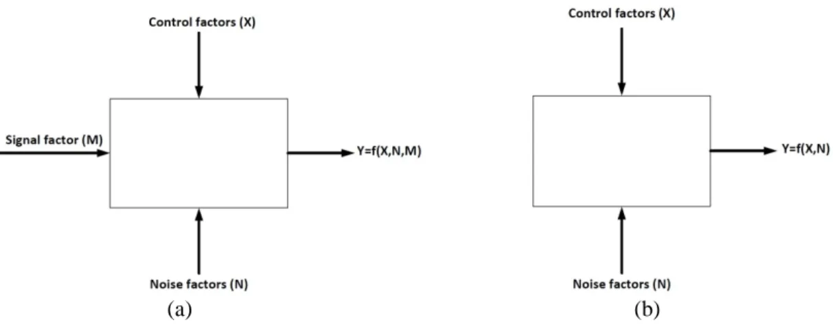
Taguchi divided the RPD methodology into two categories: static and dynamic characteristics. Static systems are defined as those desired output of the system that has a fixed target value and one attempts to obtain the value of a quality characteristic of interest as close as possible to a single specified target value. Whereas dynamic systems are those that target value depends on the input signal set and there is a relationship between response (output) and signal factor (input). This signal-response relationship is of primary importance to the performance of the system. Figure 1(a-b) denotes dynamic and static systems.
Miller and Wu (2002) criticized the terminology of Taguchi and labeled the static system as simple-response system and the dynamic system as signal-response system. They said that static and dynamic systems are applied for those systems which concerned with time whereas the simple response system and signal-response systems can concern with other input variables. They divided signal-response system into two categories: multiple target systems and measurement systems. Wu and Hamada (2001) introduced the third category as the control systems.
Because the signal-response concept plays an important role in product/process development, robust parameter design of signal-response systems (also called dynamic parameter design in Taguchi’s terminology) is an effective and powerful tool for quality improvement.
Signal-response systems ideally suppose that there is a linear relationship between the response and the signal factor. Moreover, dispersion and sensitivity are two important aspects of the signal-response system which are considered with an index such as SNR (Wu and Hamada, 2001). According to the linear assumption of relationship function, the simple linear regression model can be written as follows:
,
y= +
α β
M +ε
(1)where, M is the signal factor with predefined p levels with the value of
m
i in ith level,y
i is the response value in ith level of signal factor, E( )
ε
=0and Var( )
ε
=σ
2.It is always desirable for any signal-response system to have a small dispersion, i.e., a small
σ
2value. A large sensitivity (i.e., a largeβ
value) is also desirable. A performance measure, which convertsσ
2 andβ
in to a single measure is2
2
ln
β
ω
σ
=
(2)Taguchi proposed the dynamic SNR formula for a nominal the best response as follows: 2
2
10 log
SNR
β
σ
=
(3)(a) (b)
Figure 1. (a) Dynamic system (b) Static system
The dispersion and sensitivity are measured by
σ
2 andβ
, respectively.β
andσ
are evaluated for different combinations of control factors. It is desired that the SNR to be maximized.In contrast to Taguchi’s dynamic SNR and two-step optimization procedure, Miller and Wu (2002) developed performance measure modeling (PMM) and response function modeling (RFM) to optimize signal-response systems. PMM requires a two stage modeling. The first stage includes estimation of performance measure (PM) and second stage consists the modeling of PM as a function of control factors using estimation of PM.
RFM uses the experimental data to model the signal-response relationship as a function of the control and noise factors. The specified performance measure is then evaluated with respect to the fitted regression models. This method is an extension of the response modeling approach first recommended by Welch et al. (1990) and Shoemaker et al. (1991) for simple response applications. Wasserman (1996) presented a case study of the parameter design with dynamic characteristics by using multiple regression models. He demonstrated Taguchi’s SNR with a linear statistical model. Khattree (1996) provides a method for to estimate robust parameter design in the situation in which all of the noise variables cannot be studied simultaneously. He used the response surface approach.
Lunani, Nair and Wasserman (1997) noted that using SNR as a quality performance measure might produce inaccuracies due to a mistake to evaluate dispersion effect. They developed two graphical methods for identifying appropriate measures of dispersion, thereby avoiding interactions between the dispersion and sensitivity effects for a dynamic problem. Miller (2002) compared three methods of analyzing signal-response applications, including Miller and Wu’s (2002) approach, Taguchi method and a graphical approach proposed by Lunani, Nair and Wasserman (1997). He introduces a new graphical technique, the joint effects plot and demonstrated usefulness of the proposed method.
Lesperance and Park (2003) proposed a joint generalized linear model to evaluate the robust design of dynamic characteristics, which is based on standard regression modeling techniques. Roshan and Wu (2002) described the application of SNR in the analysis of the multiple target systems (i.e., first category of signal-response systems). Again Roshan and Wu (2002) introduced a theoretical formulation for multiple target systems and developed a practical approach for optimization which overcomes some limitations.
Wu and Yeh (2005) presented an approach to optimize multiple dynamic problems based on quality loss function. The objective is to minimize the total average quality loss for the multiple dynamic quality characteristic's experiments. Zhiyu, Zhen and Xiangfen (2006), proposed a new desirability function method for multiple robust parameter design. Their proposed method can yield better results than traditional desirability function approach. Gupta, Kulahci, Montgomery and Borrer (2009), proposed a split-plot approach to the signal-response system characterized by two variance components. They demonstrate that explicit modeling of variance components using generalized linear mixed model (GLMM) leads to more precise point estimates of important model coefficients with shorter confidence intervals within-profile variance and between-profile variance.
Dasgupta, Miller and Wu (2010), presented a robust design of measurement systems (i.e., second category of signal-response systems). They developed an integrated approach for estimation and reduction of measurement variation through a single parameter design experiment. They considered a linear signal-response relationship. Arvidsson and Gremyr (2008) prepared a literature review of conflicts and agreements on the principles of robust design. Through this review four central principles of robust design are identified: awareness of variation, insensitivity to noise factors, application of various methods, and application in all stages of a design process.
Boylan and Cho (2013), proposed a multidisciplinary RPD methodology that provides an enhanced approach for modeling multiple, mixed type quality characteristics; uses the skew normal distribution to allow for a fuller and more accurate representation of asymmetric system properties.
Boylan, Goethals and Rao Cho (2013), proposed a trade-off analysis between the cost of replication and the desired precision of generated solutions. They considered several techniques in the early stages of experimental design, using Monte Carlo simulation as a tool, for revealing potential options to the decision maker.
Yadav, Bhamare and Rathore (2010), explore the possibilities of combining both approaches into a single model and proposes a hybrid quality loss function-based multi-objective optimization model.
Truong, Shin and Jeong (2011), focus on solving the robust design (RD) problem that occurs in pharmaceutical studies in which output responses are measured over time
In general, several researches have addressed multiple static quality characteristics problems (i.e. Dasgupta, Miller and Wu (2010), Khuri and Conlon (1981), Lin, Lin and Ko (2002), Su and Tong (1997), Lu and Antony (2002), Wu (2002), Vining (1997), Tong, Su and Wang (1997,1999).
Several publications have studied the robust design problem considering the dynamic systems (i. e. Wasserman (1996), Lunani, Nair and Wasserman (1997), Miller and Wu (1996), Su and Hsieh (1998), Tsui (1999), McCaskey (1997)).
However, few studies have been concerned with optimizing the parameter design for multiple dynamic quality characteristics. Chang (2008), proposed a procedure based on desirability function to optimize multiple dynamic quality characteristics. He used the Simulated Annealing (SA) to find the best factor setting. Desirability function cannot consider variation of the observations and only focuses on the distance between responses and their targets. This fact leads to effect of noise factor and the fluctuation of the design parameters are ignored in this approach (Zhiyu, Zhen and Xiangfen (2006)). Hence, it cannot be a precise index to evaluate the results completely.
Chang (2008), used SNR of responses instead of responses values to solve the mentioned problem, in addition he used geometric mean to construct a single index for evaluating responses. However, there are some problems with his proposed approach as follows.
(i) Using geometric mean leads to face strong effect on the single aggregated index when there is a less SNR value, while other responses may have a high desirability values. Hence, analyzer ignores setting of control factors and process is rejected basically.
(ii) The effect of correlation between responses is not considered, because each response is analyzed separately. Hence, Chang’s (2008) procedure has an equal result for two processes which have similar mean and variance but different correlation. Note that, correlation between responses has a clear effect on the responses.
Similar to Chang (2008), the method proposed by Tong and Su (1997) considers TOPSIS method and focuses on SNR between responses and does not account for correlation between responses.
Tong, Wang and Houng (2001) solved the mentioned problem with desirability function and proposed the dual response surface method based on the desirability function. They first provide a regression model of responses and then calculate desirability of mean and variance. Finally, a response surface model is generated to consider the problem in two aspects of mean and variance. Their proposed approach is more reliable because of considering the responses variances. However, it does not consider the correlation between responses.
Jalili, Bashiri and Amiri (2011), applied Data Envelopment Analysis (DEA) to optimize multivariate dynamic Taguchi design. The drastic difference between the method based on the DEA and proposed method of this paper is the correlation issue. The DEA cannot consider correlation of responses, but the multivariate process
capability index can account for the correlation between response variables. Moreover, the DEA is not a parametric method, hence normality assumption of the response variables is not required in this method while the multivariate process capability index used in this paper needs the normality assumption. In spite of the differences between the DEA and multivariate process capability index, both methods are appropriate for non linear relationship between response variable and controllable factors.
Amiri, Bashiri, Mogouie and Doroudyan (2012), proposed a non-normal response optimization method based on process capability index. Their method transforms the known non normal distribution to multivariate normal distribution and then uses process capability index to optimize a multi-response problem. The difference between that method and the proposed method in this paper is the ability of the proposed method to consider unilateral quality characteristics.
He, Zhu and Park (2012), proposed a robust desirability function approach to simultaneously optimize multiple responses. Their method takes account for all values in the confidence interval rather than a single predicted value for each response and then defines the robustness measure for the traditional desirability function using the worst case strategy. They used geometric mean to aggregate calculated desirability functions. This technique has some drawbacks as mentioned before.
Awad and Kovach (2011) utilized process capability index and proposed an optimization method for multi responses problems. Their multivariate process capability index,MCpm, index is applicable if there is a target value for each response
Pal and Gauri (2010), proposed a new method that integrates multiple regression technique and Taguchi's signal-to-noise (SN) ratio concept. Two sets of experimental data were analyzed using this method. The proposed method considers total SN ratio as well as closeness of individual responses to their corresponding target values.
Hence, an efficient index which investigates a signal-response system should have two conditions. First, it should consider both location and dispersion of responses. Secondly, the proposed index should not have any relaxations about the relationship between responses and signal factor such as linearity. One of the important issues in optimization is about stage. Optimization can be applied in the both design and operation stage (for example of applying in operation stage see Sekhar and Tan (2009)). So, optimization methods which used process mean can be a suitable technique for optimization in operation stage.
1-2- Process Capability Index
Process Capability Indices (CPI) such as Cp, Cpk and Cpm are used in statistical process control to evaluate the capability of the processes in satisfying the customer’s needs. Capability index Cp is defined as the ratio of tolerance range to the spread of the process as follows:
, 6
p
USL LSL C
σ
−
= (4)
where USL and LSL are upper and lower specification limits. Also
σ
is standard deviation of quality characteristic. Sometimes, more than one quality characteristic describes the quality of a process. For analyzing the capability of these processes with correlated quality characteristics, multivariate CPIs are introduced by some researchers.In this paper to evaluate responses of a multivariate signal-response system, we use MPCNCV which have been proposed by Jalili, Bashiri and Amiri (2011). The proposed index is expressed as follows:
1
, ,
NCV
PR CV PR NCV D MPC = λ× + +β
+
(5)
where PR is process region, CV is conformance volume between the process region and modified tolerance region and NCV is non-conformance volume between the process region and modified tolerance region.
λ
is the sensitivity process capability parameter and in a bivarite response with bilateral specification limits isproposed to be 0.27 (Jalili et al., 2011). Also β is added to the first component of the MPCNCV to increase the sensitivity of the index to the processes which are completely within modified tolerance region. According to the simulations, it is better to applyβ =0.1. However, if volume of tolerance region is less than 1 it is advised to applyβ =0.05×Volume of Tolerance Region, because β =0.1 leads to overestimations of the index. Also distance between process and target is computed as
(
(
)
(
)
)
1 2 1
1
D= + µ−T ′∑− µ−T (Jalili et al., 2011).
Advantage of the MPCNCV is applicable to both unilateral and bilateral situations. Hence, when there is a unilateral response, MPCNCV can consider the problem effectively. One of the other methods which is used to consider a unilateral response is desirability function. But as mentioned before desirability function cannot consider variance of responses and only take in to account the distance between each responses with corresponding target.
Another advantage of using MPCNCV in process capability is the capability of considering correlation between responses and also its first component could consider distance between process mean and target and variation of observations simultaneously respect to traditional approaches (Jalili et al., 2011).
Hence, using process capability to evaluate the signal-response system can be useful to consider location (mean) and dispersion (variance) of observation as well as correlation of responses.
The rest of the paper is organized as follows: The proposed method is discussed in Section 2. In Section 3, a simulated dataset is applied and the performance of the proposed index is evaluated. Our concluding remarks and some future researches are given in the final section.
2- Proposed method
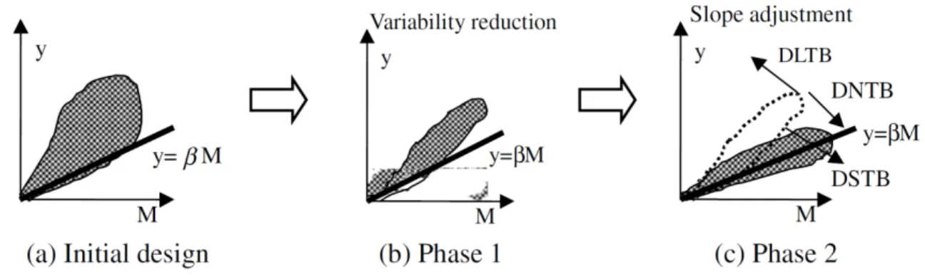
As mentioned before, to evaluate performance of the signal-response system, first a measurement index should be proposed. For example, Taguchi (1987), proposed SNR. This index considers dispersion and sensitivity of responses. Figure 2 depicts the processes of the Taguchi procedure. In this method as the first phase, variability of response decreases, and then in the second phase, the slope is brought to the target.
Figure 2. Taguchi procedure for dynamic problem (Extracted from Chang, 2008)
The target may be dynamic nominal the best (DNTB), dynamic larger the better (DLTB) or dynamic smaller the better (DSTB). In this paper, we propose a method based on process capability to evaluate performance of control factors combination. In a signal-response system, we assume there are n correlated responses in each level of signal factor. Furthermore, there are p levels for signal factor. So n×p response values should be considered.
The advantage of using process capability (PC) index in the signal-response system is that the n correlated responses in each level of signal factor can be converted to one response (process capability) which considers dispersion and sensitivity of responses without losing any properties of observations such as correlation. So
there are 1×p independent process capability indices and the optimization procedure can be done by using new independent responses.
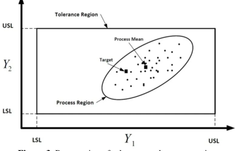
Suppose that there are two responses for a signal-response system. It is obviously that in each level of signal factor, responses should have less variability (dispersion) and distances from the targets (sensitivity). As illustrated in Figure 3, PC index try to find a parameter combination which leads to decreasing in variability and distance from target, simultaneously. In Figure 3, observed data produce a region called the process region. The upper and lower bound of responses produce a region called the tolerance region. Observations which have less variability and less distance from the target have a larger PC value. Subsequently, with modeling PCs according to the control factors, the control factors setting, which has the maximum sensitivity and minimum dispersion are obtained.
Another advantage of using PC is that it considers the effects of noise factors on responses by considering the variation of responses. Hence, proposed combination of control factors in each level of signal factor is robust to the noise factor. In this paper, just the first component of MPCNCV is considered because it includes both dispersion and sensitivity aspects.
The proposed index has the following three steps: In step 1 MPCNCV of responses in each level of the signal factor is calculated. Then, in step 2, a general model for MPCNCV according to the control factors is computed. Note that the numbers of MPCNCV models are equal to the levels of signal factor. If the levels of signal factor increase, the generated models increases and then, there are more proposed setting for considered system. Consequently more improvement for responses is available. In step 3 by an optimization method, the best levels of the control factors are obtained.
Figure 3. Presentation of tolerance and process regions
3- Numerical Example
In this section a simulated example is applied to show the performance of the proposed method. First a data set is simulated. In the simulation process, a predefined relationships between responses and control factors are used. Then, in the step 1, the process capability (MPCNCV) index for each treatment and in every level of signal factors is calculated and in the step2, a regression equation between MPCNCVand control factors is constructed for each level of signal factors. Finally, by optimizing regression equation, best level of control factors are estimated. Also the improvement of optimization will be compared by the best treatment of design matrix.
We investigate the proposed index by simulated dataset. Suppose that there are two responses
Y
1 andY
2, five controllable factorsx x x x x
1,
2,
3,
4,
5, one noise factor N and a signal factor M. According to the Equation (2), relationship function betweenY
1 and signal factor M is expressed as:1 1 1
Y
=
α β
+
M
+
ε
In numerical example, it is assumed that
α
1andβ
1 are as follows respectively:1 2 3 0.3
0.2 0.5 0.7 0.3 0.2 0.1
0.4 0.3 0.5 0.6
A B C D E
AB AC AD
BD CD DE
AN BN DN EN
α = + + − + +
+ − +
− + +
+ − +
1 2 0.1 0.2
0.4 0.3 0.1 0.5 0.2 0.7 0.2 0.1
0.5 0.5 0.2
A B C D E
AC AD BC BE
CD CE DE AN
BN CN EN
β = + − − + +
+ + + −
− + + +
− +
Furthermore, relationship between
Y
2 and signal factor M is expressed as:2 2 2
Y
=
α
+
β
M
+
ε
Also it is assumed that
α
2andβ
2 is:2 3 2 0.2
0.7 0.2 0.3 0.1
0.4 0.1 0.3 0.1 0.2 0.2 0.3 0.7
A B C D E
AB AC AD AE
BC CD CE DE
AN BN DN EN
α = + + + + +
+ + + −
+ − + +
− + +
2 2 0.7
0.4 0.2 0.8 0.1
0.3 0.2 0.7 0.4 0.2 0.3 0.2 0.1
A B C D E
AB AC AD BC
BD CD CE DE
AN BN CN EN
β = − + + − + −
+ + + +
+ + + −
+ + +
ε
is a random variable with bivariate normal distribution and E( ) ( )
ε
= 0, 0 and variance-covariance matrix1 0.1
0.1 1
∑ =
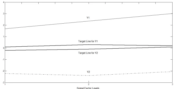
. Signal factor M has three levels of 0.1, 0.2 and 0.3.Figure 4 depicts the assumed relationship between
Y
1 ,Y
2 and M and target lines for them with a random setting for control factors. Target values for each level of the signal factor forY
1 are 0.1, 0.2 and 0.1 respectively. And these values forY
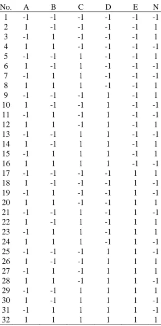
2 are -0.2, -0.1, 0.1.To consider an example, a combined array with resolution VI is used by a
2
VI6 1− design (see Table 1). 10 replicates forY
1 andY
2 in each level of signal factor are simulated.Table 1. Combined array 2VI6 1− for the numerical example
No. A B C D E N
1 -1 -1 -1 -1 -1 -1
2 1 -1 -1 -1 -1 1
3 -1 1 -1 -1 -1 1
4 1 1 -1 -1 -1 -1
5 -1 -1 1 -1 -1 1
6 1 -1 1 -1 -1 -1
7 -1 1 1 -1 -1 -1
8 1 1 1 -1 -1 1
9 -1 -1 -1 1 -1 1
10 1 -1 -1 1 -1 -1
11 -1 1 -1 1 -1 -1
12 1 1 -1 1 -1 1
13 -1 -1 1 1 -1 -1
14 1 -1 1 1 -1 1
15 -1 1 1 1 -1 1
16 1 1 1 1 -1 -1
17 -1 -1 -1 -1 1 1
18 1 -1 -1 -1 1 -1
19 -1 1 -1 -1 1 -1
20 1 1 -1 -1 1 1
21 -1 -1 1 -1 1 -1
22 1 -1 1 -1 1 1
23 -1 1 1 -1 1 1
24 1 1 1 -1 1 -1
25 -1 -1 -1 1 1 -1
26 1 -1 -1 1 1 1
27 -1 1 -1 1 1 1
28 1 1 -1 1 1 -1
29 -1 -1 1 1 1 1
30 1 -1 1 1 1 -1
31 -1 1 1 1 1 -1
32 1 1 1 1 1 1
Figure 4. Relationship between Y1 , Y2and M with a random setting for control factors with simulated data
Steps of the proposed procedure are as follows:
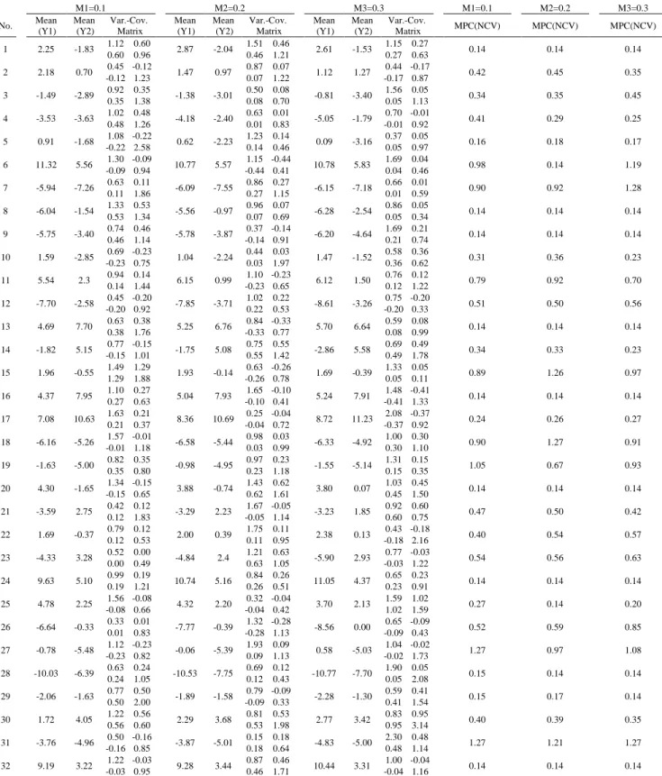
Step 1. Calculate the
MPC
NCV index for each level of signal factor M in each treatment.The mean and variance-covariance matrix of
Y
1 andY
2 are computed and the value of first component of NCVMPC for each level of signal factor M is reported in table 2. Note that the values of MPCNCV should be maximized. Hence, the factor setting which leads to maximum value of MPCNCV in each level of signal factor is desired. For example treatment 31 which contains larger value of MPCNCV in each level of signal factor can be a preferable factor setting.
Step 2. Construct the regression function between controllable factors and the
MPC
NCV .In this step according to the values ofMPCNCV, a general linear model for each level of signal factor is generated. The constructed models of MPCNCV for the numerical example are as follows:
1 0.09 0.09 0.25 0.07
0.07 0.09 0.46
PC A B AB AD
AE BD
= − + − −
− + + where M =0.1
2 0.09 0.09 0.24 0.1
0.06 0.1 0.08 0.44
PC A B AB AC
AD BD BE
= − + − −
− + − +
0.2
where M =
3 0.08 0.08 0.27
0.09 0.07 0.48
PC A B AB
BD CE
= − + −
+ − +
0.3
where M =
Where
PC
i is the process capability regression function in the ith level of signal factor.Step 3. Optimize the problem in each level of signal factor.
In this step, each of the former regression models is optimized as an objective function. The process capability model in other levels of signal factor is considered as constraints and should be capable. Hence, their values should be at least 1. For example, the optimization model for
PC
1 is expressed as:: 0.09A 0.09B 0.07AD 0.07AE 0.09BD 0.46
Max − + − − + +
. : 0.09 0.09 0.24 0.1
0.06 0.1 0.08 0.44 1
S T A B AB AC
AD BD BE
− + − −
− + − + >
0.08A 0.08B 0.27AB 0.09BD 0.07CE 0.48 1
− + − + − + >
1 A 1
− ≤ ≤
1 B 1
− ≤ ≤
1 C 1
− ≤ ≤ 1 D 1
− ≤ ≤
1 E 1
− ≤ ≤
Upper and lower bounds for control factors are 1 and -1, respectively.
Table 2. The experimental results and calculated MPCNCV index for the numerical example
M1=0.1 M2=0.2 M3=0.3 M1=0.1 M2=0.2 M3=0.3
No. Mean (Y1) Mean (Y2) Var.-Cov. Matrix Mean (Y1) Mean (Y2) Var.-Cov. Matrix Mean (Y1) Mean (Y2) Var.-Cov.
Matrix MPC(NCV) MPC(NCV) MPC(NCV) 1 2.25 -1.83 1.12 0.60 2.87 -2.04 1.51 0.46 2.61 -1.53 1.15 0.27 0.14 0.14 0.14
0.60 0.96 0.46 1.21 0.27 0.63
2 2.18 0.70 0.45 -0.12 1.47 0.97 0.87 0.07 1.12 1.27 0.44 -0.17 0.42 0.45 0.35
-0.12 1.23 0.07 1.22 -0.17 0.87
3 -1.49 -2.89 0.92 0.35 -1.38 -3.01 0.50 0.08 -0.81 -3.40 1.56 0.05 0.34 0.35 0.45
0.35 1.38 0.08 0.70 0.05 1.13
4 -3.53 -3.63 1.02 0.48 -4.18 -2.40 0.63 0.01 -5.05 -1.79 0.70 -0.01 0.41 0.29 0.25
0.48 1.26 0.01 0.83 -0.01 0.92
5 0.91 -1.68 1.08 -0.22 0.62 -2.23 1.23 0.14 0.09 -3.16 0.37 0.05 0.16 0.18 0.17
-0.22 2.58 0.14 0.46 0.05 0.97
6 11.32 5.56 1.30 -0.09 10.77 5.57 1.15 -0.44 10.78 5.83 1.69 0.04 0.98 0.14 1.19
-0.09 0.94 -0.44 0.41 0.04 0.46
7 -5.94 -7.26 0.63 0.11 -6.09 -7.55 0.86 0.27 -6.15 -7.18 0.66 0.01 0.90 0.92 1.28
0.11 1.86 0.27 1.15 0.01 0.59
8 -6.04 -1.54 1.33 0.53 -5.56 -0.97 0.96 0.07 -6.28 -2.54 0.86 0.05 0.14 0.14 0.14
0.53 1.34 0.07 0.69 0.05 0.34
9 -5.75 -3.40 0.74 0.46 -5.78 -3.87 0.37 -0.14 -6.20 -4.64 1.69 0.21 0.14 0.14 0.14
0.46 1.14 -0.14 0.91 0.21 0.74
10 1.59 -2.85 0.69 -0.23 1.04 -2.24 0.44 0.03 1.47 -1.52 0.58 0.36 0.31 0.36 0.23
-0.23 0.75 0.03 1.97 0.36 0.62
11 5.54 2.3 0.94 0.14 6.15 0.99 1.10 -0.23 6.12 1.50 0.76 0.12 0.79 0.92 0.70
0.14 1.44 -0.23 0.65 0.12 1.22
12 -7.70 -2.58 0.45 -0.20 -7.85 -3.71 1.02 0.22 -8.61 -3.26 0.75 -0.20 0.51 0.50 0.56
-0.20 0.92 0.22 0.53 -0.20 0.33
13 4.69 7.70 0.63 0.38 5.25 6.76 0.84 -0.33 5.70 6.64 0.59 0.08 0.14 0.14 0.14
0.38 1.76 -0.33 0.77 0.08 0.99
14 -1.82 5.15 0.77 -0.15 -1.75 5.08 0.75 0.55 -2.86 5.58 0.69 0.49 0.34 0.33 0.23
-0.15 1.01 0.55 1.42 0.49 1.78
15 1.96 -0.55 1.49 1.29 1.93 -0.14 0.63 -0.26 1.69 -0.39 1.33 0.05 0.89 1.26 0.97
1.29 1.88 -0.26 0.78 0.05 0.11
16 4.37 7.95 1.10 0.27 5.04 7.93 1.65 -0.10 5.24 7.91 1.48 -0.41 0.14 0.14 0.14
0.27 0.63 -0.10 0.41 -0.41 1.33
17 7.08 10.63 1.63 0.21 8.36 10.69 0.25 -0.04 8.72 11.23 2.08 -0.37 0.24 0.26 0.27
0.21 0.37 -0.04 0.72 -0.37 0.92
18 -6.16 -5.26 1.57 -0.01 -6.58 -5.44 0.98 0.03 -6.33 -4.92 1.00 0.30 0.90 1.27 0.91
-0.01 1.18 0.03 0.99 0.30 1.10
19 -1.63 -5.00 0.82 0.35 -0.98 -4.95 0.97 0.23 -1.55 -5.14 1.31 0.15 1.05 0.67 0.93
0.35 0.80 0.23 1.18 0.15 0.35
20 4.30 -1.65 1.34 -0.15 3.88 -0.74 1.43 0.62 3.80 0.07 1.03 0.45 0.14 0.14 0.14
-0.15 0.65 0.62 1.61 0.45 1.50
21 -3.59 2.75 0.42 0.12 -3.29 2.23 1.67 -0.05 -3.23 1.85 0.92 0.60 0.47 0.50 0.42
0.12 1.83 -0.05 1.14 0.60 0.75
22 1.69 -0.37 0.79 0.12 2.00 0.39 1.75 0.11 2.38 0.13 0.43 -0.18 0.40 0.54 0.57
0.12 0.53 0.11 0.95 -0.18 2.16
23 -4.33 3.28 0.52 0.00 -4.84 2.4 1.21 0.63 -5.90 2.93 0.77 -0.03 0.54 0.56 0.63
0.00 0.49 0.63 1.05 -0.03 1.22
24 9.63 5.10 0.99 0.19 10.74 5.16 0.84 0.26 11.05 4.37 0.65 0.23 0.14 0.14 0.14
0.19 1.21 0.26 0.51 0.23 0.91
25 4.78 2.25 1.56 -0.08 4.32 2.20 0.32 -0.04 3.70 2.13 1.59 1.02 0.27 0.14 0.20
-0.08 0.66 -0.04 0.42 1.02 1.59
26 -6.64 -0.33 0.33 0.01 -7.77 -0.39 1.32 -0.28 -8.56 0.00 0.65 -0.09 0.52 0.59 0.85
0.01 0.83 -0.28 1.13 -0.09 0.43
27 -0.78 -5.48 1.12 -0.23 -0.06 -5.39 1.93 0.09 0.58 -5.03 1.04 -0.02 1.27 0.97 1.08
-0.23 0.82 0.09 1.13 -0.02 1.73
28 -10.03 -6.39 0.63 0.24 -10.53 -7.75 0.69 0.12 -10.77 -7.70 1.90 0.05 0.15 0.14 0.14
0.24 1.05 0.12 0.43 0.05 2.08
29 -2.06 -1.63 0.77 0.50 -1.89 -1.58 0.79 -0.09 -2.28 -1.30 0.59 0.41 0.15 0.17 0.14
0.50 2.00 -0.09 0.33 0.41 1.54
30 1.72 4.05 1.22 0.56 2.29 3.68 0.81 0.53 2.77 3.42 0.83 0.95 0.40 0.39 0.35
0.56 0.60 0.53 1.98 0.95 3.14
31 -3.76 -4.96 0.50 -0.16 -3.87 -5.01 0.15 0.18 -4.83 -5.00 2.30 0.48 1.27 1.21 1.27
-0.16 0.85 0.18 0.64 0.48 1.14
32 9.19 3.22 1.22 -0.03 9.28 3.44 0.87 0.46 10.44 3.31 1.00 -0.04 0.14 0.14 0.14
-0.03 0.95 0.46 1.71 -0.04 1.16
By optimizing the above model, the best levels of the control factors are calculated and named as model 1 optimal setting.
1, 1, 1, 1, 0
A= − B= C= D= E=
1 1.05, 2 1.12, 3 1
PC = PC = PC =
Similar to model of
PC
1, the optimizing models ofPC
2 andPC
3 are conducted and the best levels of optimizing modelPC
2 and PC3 is obtained as follows. We call them as model 2 and 3 optimal settings respectively:1, 1, 1, 1, 0.714
A= − B= C= D= E= −
1 1, 2 1.18, 3 1.05
PC = PC = PC =
1, 1, 0.1, 1, 0.125
A= − B= C= − D= E=
1 1.06, 2 1, 3 1
PC = PC = PC =
According to the proposed levels for control factors,
Y
1 andY
2have been simulated 1000 times for three models. Note that the noise factor changes randomly between its upper and lower values. In addition, according to the results obtained by initial simulations, we select treatments 7, 15, 18, 19, 27 and 31 from experimental design which have the best results of process capability in simulated data. Then, the mean and variance of responses in optimal settings of model 1, 2 and 3 are compared with mean and variance of responses in selected treatments respect to the targets to show the better performance of the proposed method.As Table 3 shows, the variance of responses for the selected treatments is a large value and the distance of means from targets are not acceptable. Hence, these treatments do not produce an efficient response with minimum variation and distance from the target.
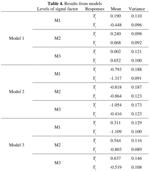
The optimal results of the models 1, 2 and 3 have been used to calculate the response mean and variance in a continuous space. The results have been shown in Table 4. Mean and variance of
Y
1 andY
2 indicate that setting of control factors obtained from the proposed method has less variance value than the selected treatments and the method is capable to bring the mean of observations to the targets.By comparing the results of Tables 3 and 4, we can conclude that distance between responses’ means and targets and variation of responses decrease considerably based on the proposed method. To demonstrate this fact, Table 5, 6 and 7 give a comparison between the selected treatments (7, 15, 18, 19, 27, and 31) and models 1, 2 and 3 optimal setting which reported before.
In these tables the percent of improvement for responses in each model are compared with the best selected treatments. The results of proposed index in Equation (6) show efficiency of the proposed approach in dynamic multi-response robust optimization.
, , * , ,
,
, , ,
i m i m i m i m bt
i m
k bt i m i m
bt
Y T Y T
IR
Y T
− − −
=
− (6)
where . .
k bt
i m
IR
is the improvement rate for the ith response in mth level of signal factor between kth model and btth treatment, Ybti m, is the best observed ith mean (variance) response value in mth level of signal factor for btth treatment,Y
* ,i mis the optimal mean (variance) value of ith response in mth signal level obtained by the proposed models and theT
i m, is the mean (variance) target of ith response of mth signal level. Note that the target value of variance for responses in the entire signal factor levels is set to zero level.Table 3. Mean and variance of selected treatments between 32 existing ones according to the NCV
MPC index value for simulated data
Signal factor levels
Responses Mean Variance
Signal factor levels
Responses Mean Variance
Treatment 7
M1 1
Y 1.096 0.105
Treatment 19
M1 1
Y 2.438 0.203
2
Y 3.142 0.259 Y2 1.956 0.097
M2 1
Y 1.208 0.103
M2 1
Y 3.069 0.218
2
Y 2.717 0.223 Y2 1.818 0.106
M3 1
Y 1.122 0.109
M3 1
Y 3.486 0.241
2
Y 2.328 0.222 Y2 1.780 0.098
Treatment 15
M1 1
Y 1.343 0.214
Treatment 27
M1 1
Y 1.528 0.107
2
Y 1.159 0.146 Y2 -0.091 0.129
M2 1
Y 1.629 0.236
M2 1
Y 2.164 0.089
2
Y 1.078 0.147 Y2 0.049 0.138
M3 1
Y 1.671 0.244
M3 1
Y 2.615 0.103
2
Y 1.078 0.126 Y2 0.229 0.147
Treatment 18
M1 1
Y 1.206 0.230
Treatment 31
M1 1
Y 1.542 0.096
2
Y 1.044 0.152 Y2 0.683 0.137
M2 1
Y 1.266 0.247
M2 1
Y 1.577 0.101
2
Y 1.551 0.133 Y2 1.411 0.152
M3 1
Y 1.154 0.230
M3 1
Y 1.431 0.099
2
Y 2.195 0.124 Y2 2.218 0.159
Table 4. Results from models
Levels of signal factor Responses Mean Variance
Model 1
M1 1
Y 0.190 0.110
2
Y -0.448 0.096
M2 1
Y 0.240 0.098
2
Y 0.068 0.092
M3 1
Y 0.002 0.121
2
Y 0.652 0.100
Model 2
M1 1
Y -0.793 0.188
2
Y -1.317 0.091
M2 1
Y -0.818 0.187
2
Y -0.864 0.123
M3 1
Y -1.054 0.173
2
Y -0.416 0.123
Model 3
M1 1
Y 0.311 0.129
2
Y -1.109 0.100
M2 1
Y 0.544 0.116
2
Y -0.803 0.089
M3 1
Y 0.637 0.146
2
Y -0.519 0.108
Consider Model 1. For example, according to the Table 4, mean of
Y
1 in the first level of signal factor is 0.190. This value for treatment 7 is 1.096 (see Table 3). So improvement rate forY
1 of model 1 respect to treatment 7 in first level of signal factor calculated as follows:1,1 1, 7
1.096 0.1 0.190 0.1 0.91 1.096 0.1
trt
IR = = − − − =
−
Note that in some levels of signal factor for responses, the distance between mean and targets is increased. For example, mean of
Y
2 in the first level of the signal factor in model 1 is−
0.448
. This value for treatment 27 is0.091
−
. Hence, its improvement rate is -1.28. Tables 5, 6 and 7 show that in most of cases, the obtained improvement rates are positive and large.Table 5. Comparison between mean and variance of the best selected treatments respect to the model 1 according to the proposed IR index
Mean
M1 M2 M3
1
Y Y2 Y1 Y2 Y1 Y2
Treatment 7 0.91 0.93 0.96 0.94 0.90 0.75 Treatment 15 0.93 0.82 0.97 0.86 0.94 0.44 Treatment 18 0.92 0.80 0.96 0.90 0.91 0.74 Treatment 19 0.96 0.88 0.99 0.91 0.97 0.67 Treatment 27 0.94 -1.28 0.98 -0.13 0.96 -3.28 Treatment 31 0.94 0.72 0.97 0.89 0.93 0.74
Variance
M1 M2 M3
1
Y Y2 Y1 Y2 Y1 Y2
Treatment 7 -0.05 0.63 0.05 0.59 -0.10 0.55 Treatment 15 0.49 0.34 0.59 0.37 0.51 0.20 Treatment 18 0.52 0.37 0.60 0.31 0.48 0.20 Treatment 19 0.46 0.01 0.55 0.13 0.50 -0.02 Treatment 27 -0.03 0.26 -0.10 0.33 -0.17 0.32 Treatment 31 -0.14 0.30 0.03 0.39 -0.21 0.37
Table 6. Comparison between mean and variance of the best selected treatments respect to the model 2 according to the proposed IR index
Mean
M1 M2 M3
1
Y Y2 Y1 Y2 Y1 Y2
Treatment 7 0.10 0.67 -0.01 0.73 -0.13 0.77 Treatment 15 0.28 0.18 0.29 0.35 0.27 0.47 Treatment 18 0.19 0.10 0.04 0.54 -0.10 0.75 Treatment 19 0.62 0.48 0.65 0.60 0.66 0.69 Treatment 27 0.37 -9.24 0.48 -4.13 0.54 -3.01 Treatment 31 0.38 -0.27 0.26 0.49 0.13 0.76
Variance
M1 M2 M3
1
Y Y2 Y1 Y2 Y1 Y2
Treatment 7 -0.79 0.65 -0.81 0.45 -0.58 0.45 Treatment 15 0.12 0.38 0.21 0.16 0.29 0.02 Treatment 18 0.18 0.40 0.24 0.08 0.25 0.01 Treatment 19 0.07 0.06 0.14 -0.16 0.28 -0.25 Treatment 27 -0.76 0.29 -1.10 0.11 -0.67 0.17 Treatment 31 -0.96 0.34 -0.86 0.19 -0.74 0.23
Table 7. Comparison between mean and variance of the best selected treatments respect to the model 3 according to the proposed IR index
Mean
M1 M2 M3
1
Y Y2 Y1 Y2 Y1 Y2
Treatment 7 0.79 0.73 0.66 0.75 0.47 0.72 Treatment 15 0.83 0.33 0.76 0.40 0.66 0.37 Treatment 18 0.81 0.27 0.68 0.57 0.49 0.70 Treatment 19 0.91 0.58 0.88 0.63 0.84 0.63 Treatment 27 0.85 -7.33 0.82 -3.72 0.79 -3.81 Treatment 31 0.85 -0.03 0.75 0.53 0.60 0.71
Variance
M1 M2 M3
1
Y Y2 Y1 Y2 Y1 Y2
Treatment 7 -0.23 0.61 -0.12 0.60 -0.33 0.51 Treatment 15 0.40 0.31 0.51 0.39 0.40 0.14 Treatment 18 0.44 0.34 0.53 0.33 0.37 0.13 Treatment 19 0.37 -0.03 0.47 0.16 0.39 -0.10 Treatment 27 -0.21 0.22 -0.30 0.36 -0.41 0.27 Treatment 31 -0.35 0.27 -0.15 0.41 -0.47 0.32
Table 8 includes responses’ mean and optimal setting of control factors in three models. Figure 5 depicts the mean of
Y
1 andY
2 according to the optimal setting. As Figure 5 shows, profiles ofY
1 andY
2have less distance from target in randomly levels of the noise factor for three models. So, optimum setting which are obtained from three models could decrease distance of mean from the target in all of the signal factor levels.Table 8. Optimum setting obtained from three models
Levels of Control factors Mean
Y
1 MeanY
2A B C D E M1=0.1 M2=0.2 M3=0.3 M1=0.1 M2=0.2 M3=0.3 Model 1 -1 1 1 1 0 0.190 0.240 0.002 -0.448 0.068 0.652 Model 2 -1 1 1 1 -0.714 -0.793 -0.818 -1.054 -1.317 -0.864 -0.416 Model 3 -1 1 -0.1 1 0.125 0.311 0.544 0.637 -1.109 -0.803 -0.519
(a)
73
(b)
(c)
Figure 5. Profile of Y1 and Y2according to the proposed setting (a) Model 1 (b) Model 2 (c) Model 3
Figure 6 presents a comparison between process mean, targets and variations of model 1 as the best model and treatment 27 as the best initial treatment. In the mentioned figure, Yijis mean for ith response in jth level of
signal factor. Also Vij is variance for ith response in jth signal factor level.
Results show the efficiency of the proposed method to obtain the setting of control factors. However, distance between process mean and its target and variance for
Y
2 are increased a little, but variation and distance between process mean and the target forY
1 are decreased considerably.4- Conclusions
In this paper, a new method based on the process capability index is proposed to optimize multivariate signal-response systems. By using multivariate process capability index, location and dispersion of signal-responses can be considered with a single measurement (PC) in each level of the signal factor. Finally, PC is modeled as a general linear model in each level of signal factor according to the control factors. Optimum levels of control factors are obtained by solving optimization models of control factors in each level of signal factor. The
simulated results show the efficiency of the proposed approach considering the improvement ratio index. Determination of Pareto optimal solutions for all levels of signal factor using multi objective optimization method can be studied as a related future research.
Figure 6. Comparison between process mean and targets of Y1 and Y2 as well as variance of them for model 1 and treatment 27
References
Amiri, A., Bashiri, M., Mogouie, H., & Doroudyan, M. H. (2012). “Non-normal multi-response optimization by multivariate process capability index”, Scientia Iranica, 19 (6), pp. 1894-1905.
Arvidsson, M., & Gremyr, I. (2008). “Principles of robust design methodology”, Quality and Reliability Engineering International, 24 (1), pp. 23-35.
Awad, M. I., Kovach, J. V. (2011). “Multiresponse optimization using multivariate process capability index”, Quality and Reliability Engineering International, 27 (4), pp. 465-477.
Boylan G. L., Cho B. R. (2013). “Solving the Multidisciplinary Robust Parameter Design Problem for Mixed Type Quality Characteristics under Asymmetric Conditions”, To appear in Quality and Reliability Engineering International.
Boylan, G. L., Goethals, P. L., & Rae Cho, B. (2013). “Robust parameter design in resource-constrained environments: An investigation of trade-offs between costs and precision within variable processes”, Applied Mathematical Modelling, 37 (4), pp. 2394-2416.
Chang H. H. (2008). “A data mining approach to dynamic multiple responses in Taguchi experimental design”, Expert Systems with Applications, 35 (3), pp. 1095-1103.
Dasgupta T., Miller A., Wu C. F. J. (2010). “Robust design of measurement systems”, Technometrics, 52(1), pp. 338-346.
Gupta S., Kulahci M., Montgomery D. C., Borror C. M. (2009). “Analysis of signal-response systems using generalized linear mixed models”, Quality and Reliability Engineering International, 26 (4), pp. 375-385.
He, Z., Zhu, P. F., Park, S. H. (2012). “A robust desirability function method for multi-response surface optimization considering model uncertainty”, European Journal of Operational Research, 221 (1), pp. 241-247. Jalili M, Bashiri M, Amiri A. (2011). “A data envelopment analysis method for optimizing multi-response problem by dynamic Taguchi method”, In Proceedings of ICCS-11, Lahore, Pakistan, Vol. 21, pp. 209-222. Jalili M, Bashiri M, Amiri A. H. (2010). “A new multivariate process capability index under both unilateral and bilateral quality characteristics”, Quality and Reliability Engineering International, 28 (8), pp. 925-941 (2012). Khattree R. (1996). “Robust parameter design: A response surface approach”, Journal of Quality Technology”, 28 (2), pp. 187-198 .
Khuri A. I., Conlon M. (1981). “Simultaneous optimization of multiple responses represented by polynomial regression functions”, Technometrics, 23 (4), pp. 363-375.
Lesperance M. L., Park S. M. (2003). “GLMs for the analysis of robust design with dynamic characteristics”, Journal of Quality Technology, 35 (3) pp. 253−263.
Lin C. L, Lin J. L, Ko T. C. (2002). “Optimization of the EDM process based on the orthogonal array with fuzzy logic and grey relational analysis method”, International Journal of Advanced Manufacturing Technology, 19 (4), pp. 271-277.
Lu D, Antony. (2002). “Optimization of multiple responses using a fuzzy-rule based inference system”, International Journal of Production Research, 40 (7), pp. 1613-1625.
Lunani M, Nair V. N. Wasserman G. S. (1997). “Graphical methods for robust design with dynamic characteristics”, Journal of Quality Technology, 29 (3), pp. 327-338.
McCaskey S. D, Tsui K. L. (1997). “Analysis of dynamic design experiments”, International Journal of Production Research, 35 (6), pp. 1561-1574.
Miller A, Wu C. F. J. (1996). “Commentary on Taguchi’s parameter design with dynamic characteristics”, Quality and Reliability Engineering International, 12 (2), pp. 75-78.
Miller A. (2002). “Analysis of parameter design experiments for signal-response systems”, Journal of Quality Technology, 34 (2), pp. 39−151.
Miller, A. and Wu, C. F. J. (2002). “Parameter design for signal-response systems: a different look at Taguchi’s dynamic parameter design”, Statistical science; 11 (2), pp. 122-136.
Pal, S., & Gauri, S. K. “Multi-Response Optimization Using Multiple Regression–Based Weighted Signal-to-Noise Ratio (MRWSN)”, Quality Engineering, 22 (4), pp. 336-350.
Roshan J., Wu C. F. J. (2002). “Performance measures in dynamic parameter design”, Journal of Japanese Quality Engineering Society 10, pp. 82-86.
Roshan J., Wu C. F. J. (2002). “Robust parameter design of multiple target systems”, Technometrics, 44 (4), pp. 338-346.
Sekhar, S. C., and L. T. Tan, (2009). "Optimization of cooling coil performance during operation stages for improved humidity control." Energy and Buildings 41(2), pp.229-233.
Shoemaker A. C., Tsui K. L., Wu C. F. J., (1991). “Economical experimentation method for robust design”, Technometrics; 33 (4), pp. 415-427.
Su C. T, Hsieh K. L. (1998). “Appling neural network approach to achieve robust design for dynamic quality characteristics”, International Journal of Quality and Reliability Management, 15 (5), pp. 509-519.
Su C. T, Tong L. I. (1997). “Multi-response robust design by principal component analysis”, Total Quality Management, 8 (6), pp. 409-416.
Taguchi, G (1987). “System of experimental design”, Unipub/Kraus Int, White Plains, NY.
Tong L. I, Su C. T., Wang C. H. (1997). “The optimization of multiresponse problems in the Taguchi method by fuzzy multiple attribute decision making”, Quality and Reliability Engineering International, 13 (1), pp. 25-34.
Tong L. I., Wang C. H., Houng J. Y., Cen JY. (2001). “Optimizing dynamic multiresponse problems using the dual-response-surface method”, Quality Engineering, 14 (1), pp. 115-125.
Tong, L. I., Su, C. T., & Wang, C. H. (1997). “The optimization of multi-response problems in the Taguchi method”, International Journal of Quality & Reliability Management, 14 (4), pp. 367-380.
Truong, N. K. V., Shin, S., Jeong, S. H. (2011). “Robust design modelling and optimisation using response surface methodology and inverse problem”, International Journal of Experimental Design and Process Optimisation, 2 (3), pp. 202-220.
Tsui K. L. (1999). “Modeling and analysis of dynamic robust design experiments”, IIE Transactions, 31 (12), pp. 1113-1122.
Tsui K. L. (1999). “Robust design optimization for multiple characteristic problems”, International Journal of Production Research, 37 (2), pp. 433-445.
Vining G. G. (1998). “A compromise approach to multiresponse optimization”, Journal of Quality Technology, 30 (4), pp. 309-313.
Wasserman G. S. (1996). “Parameter design with dynamic characteristics: a regression perspective”, Quality and Reliability Engineering International”, 12 (2), pp. 113−117.
Welch, W. J. ,Yu T. K. , Kang S. M. , Sacks J. (1990). “Computer experiments for quality control by parameter design”, Journal of Quality Technology; 22 (1), pp. 15-22.
Wu F. C. (2002). “Optimization of multiple quality characteristics based on percentage reduction of Taguchi’s quality loss”, International Journal of Advanced Manufacturing Technology, 20 (10), pp. 749-753.
Wu F. C., Yeh C. H. (2005). “Robust design of multiple dynamic quality characteristics”, International Journal of Advanced Manufacturing Technology; 25 (5-6), pp. 579-588.
Wu, C. F. J. and Hamada, M. (2001). “Experiments: Planning, analysis, and parameter design optimization”, John Wiley & Sons Inc.
Yadav, O. P., Bhamare, S. S., & Rathore, A. (2010). “Reliability‐based robust design optimization: A multi‐objective framework using hybrid quality loss function”, Quality and Reliability Engineering International, 26 (1), pp. 27-41.
Zhiyu, Z., Zhen, H. E., & Xiangfen, K. (2006). “A new desirability function based method for multi-response robust parameter design”, International Technology and Innovation Conference.