Estimating Process Capability Indices Using Univariate g and h Distribution

Summer 2011 

Estimating Process Capability Indices Using Univariate g and h

Distribution

Nandini Das1

SQC&OR unit, Indian Statistical Institute, Kolkata, India [email protected]

ABSTRACT

Process capability of a process is defined as inherent variability of a process which is running under chance cause of variation only. Process capability index is measuring the ability of a process to meet the product specification limit. Generally process capability is measured by 6

assuming that the product characteristic follows Normal distribution. In many practical situations the product characteristics do not follow normal distribution. In this paper, we describe an approach of estimating process capability assuming generalised g and h distribution proposed by Tukey.

Keywords: Process Capability; Tukey Univariate g and h Distribution

1. INTRODUCTION

The objective of implementation of Statistical Process control is two-fold. One is to reduce variability of product characteristic through eliminating assignable causes of variation from the process. Another is to measure the ability of the process to meet the product specification. First one is achieved by using control chart and second one is obtained by process capability analysis. In this work we will deal with process capability analysis.

Process capability is a measure of natural variability of the product characteristic inherent by the process when it is running under chance cause of variation only. It is commonly measured as 6. The basic assumption behind this measure is that the product characteristic follows Normal distribution. Since for Normal distribution with parameter µ and , 99.73% of the observations lie within the limit (µ- 3, µ+ 3), it is quite reasonable to assume a measure variability as 6 = {(µ+ 3) – (µ- 3)}.

Various measures for Process Capability indices are used by quality control practitioners, such as:

Cp = 

when both

given

CpU =



when only

CpL =



when only

where µ and  are estimated by process average ( ) and process standard deviation (s), and U and L are the upper and lower specification limits, respectively.

Kane (1986) gave the first comprehensive interpretations of these indices. Kaminsky et al (1998) gave their critical comments on the uses of these indices, and suggested a future measurement. For detailed information on process capability indices and recent developments, see Johnson and Kotz (1993), Kotz and Lovelace (1998), Kotz and Johnson (2000) and Rodriguez (1992). In addition, Spiring et al. (2003) provided an extensive bibliography on process capability indices.

Since assumption of normality may not be valid in all practical situations use of the abovementioned measures may lead to erroneous conclusion. We have several references on non-normal process capability. Munechika (1992) provided several examples of machining processes that are inherently nonnormal. Somerville and Montgomery (1997) elaborated the effects of nonnormality on the yield of a process that is assumed normal. Kocherlakota et al. (1992) gave detailed information on the effects of nonnormality on PCIs.

One approach to handle non-normal data is to make a suitable transformation so that the transformed variable follows normal distribution and then use of normal process capability indices. But the main difficulty of this approach is to find the suitable transformation. Another approach is to make use of generalised family of distributions. Clements (1989) and Rodriguez (1992) showed the use of Pearson system; Farnum (1997), Polansky et al. (1998) and Pyzdek (1995) used all Johnson system; Castagliola (1996) used Burr distribution; Kocherlakota et al. (1992) used Edgeworth series distributions and Pal (2004) used generalised lambda distribution. Following are the references where some specific non-normal probability distribution is used. Somerville and Montgomery (1997) used t, gamma, and lognormal; Mukherjee and Singh (1998) showed use of Weibull and Sundaraiyer (1996) used inverse Gaussian distribution.

While dealing with non-normal data measure of process capability is taken as Up – Lp instead of 6, where Up is upper pth percentile and Lp is lower pth percentile and p is taken as 0.00135. The logic behind it is that µ+ 3 is upper 99.865th percentile and µ- 3 is 0.135th percentile of normal distribution. Hence in this case the main task is to estimate Up and Lp by fitting a generalised distribution.

In this article we will show use of univariate g and h distribution to estimate process capability and the corresponding indices which can be used for both normal and non-normal distribution.

2. UNIVARIATE g and h DISTRIBUTION

Tukey (1977) introduced a family of distributions called g and h family based on a transformation of a standard normal variable. Let Z denote a standard normal variable, then the g and h distribution of a univariate normal random variable Ygh is defined through the following transformation of Z

Ygh(Z) = A + B /

,

govern the skewness and elongation of Ygh, respectively.

The g and h family of distributions was extensively studied by Hoaglin (1985) and Martinez and Iglewicz (1984). Due to its appealing attributes in shape it has been getting popular for handling different real life data. Despite its complex mathematical form, percentage points of the density function can be obtained numerically using various computer software packages. Hoaglin (1985) and Martinez and Iglewicz (1984) studied the properties of this family using computer packages. Majumder and Ali (2008) also described various features of this family of distributions. The most important and useful characteristic of the gh family of distributions is that this family includes several known theoretical probability distributions like, Normal, Log-Normal, Cauchy, t, Uniform,

2, Exponential, Logistic, and Gamma. In fact, many of the other families of distributions like Pearson curve and Johnson curve can be fitted closely to g and h distribution (see Hoaglin (1985)). A quantile function is defined as the inverse of the (cumulative) distribution function

U = Fx(x│ ) for a (continuous) random variable X (here θis a vector of parameters).

So the quantile function is

X = Qx(u│ ) = Fx-1(u│ ). (2)

The quantile function of the generalized g and h distribution (MacGillivray and Cannon (2000)) is

Qx(u│ µ, , g, h) = A + B Zu(1+ c ) / , (3)

where, Zu is the uth standard normal quantile, A and B > 0 are location and scale parameters, g measures skewness in the distribution, h > 0 measures of kurtosis (in the general sense of peakedness/tailedness) of the distributions, and c is a constant chosen to help produce proper distributions. MacGillivray and Cannon recommended assuming the value for c as 0.8 for real life data.

2.1. Estimation of the constants g and h

The density of gh distribution can only be expressed as an implicit function. Thus it requires numerical computation to obtain the estimates of A, B, g and h.

Majumder and Ali (2008) described different methods for estimating g and h. Hoaglin (1985) gave the quantile method, Martinez and Iglewicz (1984) gave method of moments and Rayner and MacGillivray (2002) provided maximum likelihood method for estimating these parameters.

Hoaglin’s (1985) idea is to estimate the parameter g, first directly from the quantiles by the following equation

g

= - log

and then to estimate A and h by fitting the following regression line

ln

= A + h

.

B can be estimated by the following relationship

x

– x

=

(

-

1)

,

where A is the intercept and h is the slope of the line and xp and zp are pth quantiles of the data and standard normal distribution, respectively. Thus estimate of h is the estimate of the slope of the above regression line.

Martinez and Iglewicz (1984) derived the expression for nth order raw moment of the g and h distribution as

E(Y) = _√

(

-

1)

,

0

h

1,

E(Yn) = _√

∑

1

, g

0

,

0

h

1

/n

If m1 and m2 are the first and second moments around zero of the data then we can estimate g and h by solving the following equations E(Y) = m1 and E(Y2 ) = m2.

Because of the complex nature of the equations, it is quite difficult to have a closed form of the solution. Using computer system one can numerically solve the equations. But this is still a tedious job even for a computer system. Majumder and Ali provided a simpler method for solving these equations. They showed that g and h are almost linearly related.

From the equation E(Y) = m1 it is possible to generate number of data pairs (g, h). Based on this data we can have the least square estimate of α and β where

g = α + βh. (9)

Then putting this value of g in the equation E(Y2 ) = m2 , we can numerically solve the equation for

h. Once we have the estimated value of h, putting this value in the equation E(Y) = m1 we can then numerically solve for g.

They further noticed that for smaller values of the moments the solutions are very close. But for the larger values of the moments the solutions are quite close but not as close to the actual values as desirable. We can solve this problem by changing the scale of data since the variations of data does not affect the shape such as skewness and elongation. After changing the scale of data we can estimate the parameters g and h using this method and apply this to the original data.

Rayner and MacGillivray (2002) provided maximum likelihood estimation method for g and h. It is quite straightforward to obtain an expression for likelihood from a distribution specified by the quantile function Qx (u | θ), but only in terms of the inverse quantile functions (xi | θ). For a simple random sample x1 . . . xn taken from generalized g and h distributions we obtain

L( │ x1, . . . , xn ) = ∏ │ )

= ∏ (xi│

= (∏ | )│ ))-1.

Hence,

|

 √  /

=

(

)

(

1+ h

.

They provided some numerical methods to solve this function. After estimating the parameters one may check the goodness of fit by Q-Q plot or using 2 _{goodness of fit.}

2.2. Estimating process capability using g and h distribution

The following steps are recommended to estimate the process capability:

Step 1: Collect a sample of at least 100 observations on the relevant quality characteristic.

Step 2: Estimate the parameters A, B, g and h by using any of the above methods. Verify the goodness of fit.

Step 3: Obtain the value of Up and Lp where Up and Lp are the upper and lower pth percentile where

p = 0.00135, using the quantile function of g and h distribution by putting estimates of the parameters obtained from the data.

Step 4: Obtain the estimate of process capability as Up - Lp.

Step 5: Obtain the process capability indices as follows:

Cp = when both U and L are given 

CpU = when only U is given

CpL = when only L is given

where, M is the median or 50th percentile of the fitted g and h distribution.

3. NUMERICAL EXAMPLE

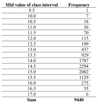
Consider the well-known data on the lengths (mm) of 9440 beans (Kendall and Stuart (1963)). The frequency distribution of the data is given in Table 1.

Hoaglin (1985) analysed the data very elaborately to fit the g and h distribution. He has obtained the following estimates of the parameters: = 14.494, = 0.815, = - 0.205, and = 0.04. He has checked the adequacy of fitting by Q-Q plot and the residual between the bin boundary and the fitted X with the equation

X 14.494 – 3.974 ( . - 1) . (11)

Table 1 Frequency distribution of bean length (in mm) data

Mid value of class interval Frequency

9.5 1 10.0 7 10.5 18 11.0 36 11.5 70 12.0 115 12.5 199 13.0 437 13.5 929 14.0 1787 14.5 2294 15.0 2082 15.5 1129 16.0 275 16.5 55 17.0 6

Sum 9440

The pth quantile is

Qp = 14.494 – 3.974 ( . - 1) .

.

Taking p = 0.00135, we have Up = 16.6795 (putting Zp = 3) and Lp = 10.4515 (putting Zp = -3). Then,

Estimated Process capability using g and h distribution = 6.228 (= Up – Lp) Estimated Process capability using normal distribution = 5.4689 (= 6)

Having Upper specification limit = 15 mm and Lower specification limit = 10 mm, we have Process capability index using g and h distribution is Cp = = 1.25, and Process capability index using normal distribution is Cp =  = 1.09.

Hence it can be concluded that using traditional process capability index gives an underestimate relative to using g and h distribution.

4. CONCLUSSION 

Traditional process capability indices can give misleading indications of a process’ ability to meet specification limits when the process measurements cannot be adequately described by a normal distribution. The generalized g and h distribution is very useful for modelling non-normal process data. This distribution provides a wide variety of curve shapes. Compared to the other alternative approaches like fitting Pearson or Johnson family of distribution curves, this distribution gives some direct formula for quantile which makes the computational procedure simpler and more flexible. In this article, we have described the procedure for using this distribution in computing generalized

process capability indices for a non-normal process. Generalising this idea, one can compute multivariate process capability by using multivariate quantile and Multivariate g and h distribution.

REFERENCES

[1] Castagliola P. (1996), Evaluation of nonnormal capability indices using Burr’s distributions; Quality Engineering 8(4); 587–593.

[2] Clements J.A. (September 1989), Process capability calculations for non-normal distributions; Quality Progress; 95–100.

[3] Farnum N.R. (1997), Using Johnson curves to describe nonnormal process data; Quality Engineering 9(2); 329–336.

[4] Hoaglin D.C. (1985), Summarizing shape numerically: The g-andh distributions. In: Hoaglin D.C., Mosteller F., and Tukey J.W. (Eds.), Exploring Data Tables, Trends and Shapes. Wiley, New York. [5] Johnson N.L., Kotz S. (1993), Process Capability Indices; John Wiley & Sons.

[6] Kaminsky F.C., Dovich R.A., Burke R.J. (1998), Process capability indices: now and in the future; Quality Progress; 10, 445-453.

[7] Kane V.E. (1986), Process capability indices; Journal of Quality Technology 18; 41-52.

[8] Kendal M.G., Stuart A. (1963), The advanced theory of statistics; vol-I, 2nd ed. London: Charles Griffin and Company Limited.

[9] Kocherlakota S., Kocherlakota K., Kirmani S.N.A.U. (1992), Process capability indices under nonnormality; Int. J. Math. Statist. Sci.1 (2); 175–210.

[10] Kotz S., Johnson N.L. (2002), Process capability indices - a review; Journal of Quality Technology 34(1); 2-19.

[11] Kotz S., Lovelace C. (1998), Introduction to Process Capability Indices; Arnold, London, UK.

[12] MacGillivray H.L., Cannon W.H. (2000), Generalizations of the g and-h distributions and their uses; Unpublished thesis.

[13] Majumder M.m.A, Ali M.M. (2008), a comparison of methods of estimation of parametersof Tukey’s gh family of distributions; Pak. J. Statist. Vol. 24(2); 135-144.

[14] Martinez J., Iglewicz B. (1984), Some properties of the Tukey g-andh family of distributions; Communications in Statistics—Theory and Methods 13(3); 353–369.

[15] Mukherjee S.P., Singh N.K. (1998), Sampling properties of an estimator of a new process capability index for weibull distributed quality characteristics; Quality Engineering 10; 291- 294.

[16] Munechika M. (1992), Studies on process capability in machining processes; Reports of Statistical Applied research JUSE 39; 14–29.

[17] Pal S. (2004), Evaluation of normal process capability indices using generalized lambda Distribution; Quality Engineering, 17; 77-85.

[18] Polansky A.M., Chou Y.M., Mason R.L. (1998), Estimating process capability indices for a truncated distribution; Quality Engineering 11(2); 257–265.

[19] Pyzdek T. (1995), Why normal distributions aren’t [all that normal]; Quality Engineering 7; 769–777. [20] Rayner G.D, MaCgillivray H.L. (2002), Numerical maximum likelihood estimation for the g-and-k

and generalized g-and-h distributions; Statistics and Computing 12; 57–75.

[21] Rodriguez R.N. (1992), Recent developments in process capability analysis; Journal of Quality Technology 24; 176–186.

[22] Somerville S.E., Montgomery D.C. (1997), Process capability indices and non-normal distributions; Quality Engineering 9(2); 305–316.

[23] Spiring, F., Leung B., Cheng S., Yeung A. (2003), A bibliography of process capability papers; Quality and Reliability Engineering International 19(5); 445-460.

[24] Sundaraiyer V.H. (1996), Estimation of a process capability index for inverse Gaussian distribution; Communications in Statistics—Theory and Methods 25; 2381–2398.

[25] Tukey J.W. (1977), Modern techniques in data analysis; NSF Sponsored Regional Research Conference, Southeastern Massachusetts University, North Dartmouth, Massachusetts.