Quartic B-Spline Collocation Method for Fifth Order
Boundary Value Problems
K.N.S.Kasi Viswanadham
Department of Mathematics National Institute of TechnologyWarangal – 506004 (INDIA)
Y.Showri Raju
Department of Mathematics National Institute of TechnologyWarangal – 506004 (INDIA)
ABSTRACT
A finite element method involving collocation method with quartic B-splines as basis functions have been developed to solve fifth order boundary value problems. The fifth order and fourth order derivatives for the dependent variable are approximated by the central differences of third order derivatives. The basis functions are redefined into a new set of basis functions which in number match with the number of collocated points selected in the space variable domain. The proposed method is tested on four linear and two non-linear boundary value problems. The solution of a non-linear boundary value problem has been obtained as the limit of a sequence of solutions of linear boundary value problems generated by quasilinearization technique. Numerical results obtained by the present method are in good agreement with the exact solutions available in the literature.
Keywords
Collocation Method; Quartic B-spline; Basis Function; Fifth Order Boundary Value Problem; Absolute Error.
1. INTRODUCTION
In this paper we developed a collocation method with quartic B-splines as basis functions for getting the numerical solution of the general linear fifth order boundary value problem ao(x)y(5)(x)+ a1(x)y(4)(x)+ a2(x)y’’’(x) + a3(x)y’’(x)+ a4(x)y’(x) + a5(x)y(x) = b(x), c < x < d (1) subject to the boundary conditions
y(c) = A0 , y(d) = B0, y’(c) = A1, y’(d) = B1, y’’(c) = A2, (2) where A0 , B0 , A1 , B1 , A2 are finite real constants and a0(x), a1(x), a2(x), a3(x), a4(x), a5(x) and b(x) are all continuous functions defined on the interval [c,d].
Generally, these types of differential equations arise in the mathematical modelling of viscoelastic fluids [1, 2]. The existence and uniqueness of the solution for these types of problems have been discussed in Agarwal [3].
Over the years, there are several authors who worked on these types of boundary value problems by using different methods. For example, Caglar et al.[4] solved fifth order special case boundary value problems by collocation method with sixth degree B-splines. They divided the domain into n subintervals by means of n+1 distinct points. They approximated the solution using the given five boundary conditions and the residual is made equal to zero at the inner collocation points only. Ghajala and Shahid [5] solved a special fifth order boundary value problems using sixth degree spline curves. Lamini et al.[6] developed two methods for the solution of the special fifth order boundary value problems.
Further, the fifth order boundary value problems were investigated by Khan [7] using finite difference methods and Wazwaz [8] by means of adomian decomposition methods. Recently, Khan et al. [9] presented a class of methods based on non-polynomial sextic spline functions for the solution of a special fifth-order boundary-value problem . El-Gamel [10] employed the Sinc-Galerkin method to solve the fifth-order boundary value problems. Noor et al. [11] applied the homotopy perturbation method for solving the fifth-order boundary value problems. Viswanadham et al. used sextic and quintic B-splines to solve fifth order special case boundary value problems [12, 13]. The use of spline functions in the context of fifth-order boundary-value problems were studied by Fyfe [14], who used quintic polynomial spline functions to develop consistency relation connecting the values of solution with fifth-order derivative at the respective nodal points. Zhao-Chun Wu [15] and Juan Zhang [16] solved fifth order boundary value problems using variational iteration method.
The above studies are concerned to solve fifth order boundary value problems by using quintic or sextic B-splines. In this paper, quartic B-splines as basis functions have been used to solve the boundary value problems of the type (1)-(2). In section 2 of this paper, the justification for using the collocation method has been mentioned. In section 3, the definition of quartic B-splines has been described. In section 4, description of the collocation method with quartic B-splines as basis functions has been presented and in section 5, solution procedure to find the nodal parameters is presented. In section 6, numerical examples of both linear and non-linear boundary value problems are presented. The solution of a nonlinear boundary value problem has been obtained as the limit of a sequence of solutions of linear boundary value problems generated by quasilinearization technique [17]. Finally, the last section is dealt with conclusions of the paper.
2. JUSTIFICATION FOR USING
COLLOCATION METHOD
otherwise
Further, the collocation method is the easiest to implement among the variational methods of FEM. When a differential equation is approximated by mth order B-splines, it yields (m+1)th order accurate results [19]. Hence this motivated us to solve a fifth order boundary value problem of type (1)-(2) by collocation method with quartic B-splines as basis functions.
3. DEFINITION OF QUARTIC
B-SPLINES
The cubic B-splines are defined in [20, 21]. In a similar analogue, the existence of the quartic spline interpolate s(x) to a function in a closed interval [c, d] for spaced knots (need not be evenly spaced)
c = x0 < x1 < x2 < … < xn-1 < xn = d
is established by constructing it. The construction of s(x) is done with the help of the quartic B-Splines. Introduce eight additional knots x-4, x-3, x-2, x-1, xn+1, xn+2, xn+3 and xn+4 such that
x-4 < x-3 < x-2 < x-1 < x0 and xn < xn+1 < xn+2 < xn+3 < xn+4. Now the quartic B-splines Bi(x) are defined by
0 ) ( ) ( ) ( 3 2 ' 4 i i r r r i x x x xB
x
[
x
i2,
x
i3]
,
0
,
)
(
)
(
44
x
x
x
x
rr
and ( ) 3( ). 2
i i r r x x x It can be shown that the set {B-2(x), B-1(x), B0(x), …, Bn(x), Bn+1(x)} forms a basis for the space
S
4(
)
of quartic polynomial splines. The quartic B-splines are the unique non-zero splines of smallest compact support with knots at x-4 < x-3 < x-2 < x-1 < x0 <…< xn < xn+1 < xn+2 < xn+3 < xn+4.4. DESCRIPTION OF THE METHOD
To solve the boundary value problem (1)-(2) by the collocation method with quartic B-splines as basis functions, we define the approximation for y(x) as)
(
)
(
1 2x
B
x
y
j n j j
(3)
where αj ’
s are the nodal parameters to be determined. In the present method, the internal mesh points x1, x2, …, xn-1 are selected as the collocation points. In collocation method, the number of basis functions in the approximation should match with the number of selected collocation points [18]. Here the number of basis functions in the approximation (3) is n+4, where as the number of selected collocation points is n-1. So, there is a need to redefine the basis functions into a new set of basis functions which in number match with the number of selected collocation points. The procedure for redefining the basis functions is as follows:
Using the quartic B-splines described in section 3 and the Dirichlet boundary conditions of (2), we get the approximate solution at the boundary points as
0 0 1
2
0
)
(
)
(
)
(
c
y
x
B
x
A
y
j j j
(4). ) ( ) ( ) ( 0 1 2 B x B x y d
y j n
n n j
j
n
(5)Eliminating α-2 and αn+1 from the equations (3), (4) and (5), we get the approximation for y(x) as
( ) ( ) ( )
1
1 x P x
w x y j n j j
(6) where ) ( ) ( ) ( ) ( ) ( 1 1 0 2 0 2 0
1 B x
x B B x B x B A x w n n n and , (x) ) (x ) ( ) ( ), ( ), ( ) ( ) ( ) ( ) ( 1 n 1 2 0 2 0 n n n j j j j j j B B x B x B x B x B x B x B x B x P
Using the Neumann boundary conditions of (2) to the approximate solution y(x) in (6), we get
y’(c) = y’(x0) = w1’(x0) + α-1P’-1(x0) + α0P’0(x0) + α1P’1(x0)
= A1 (7)
y’(d) = y’(xn) = w1 ’
(xn) + αn-2P ’
n-2(xn) + αn-1P ’
n-1(xn)
+ αnP’n(xn) =B1. (8) Now, eliminating α-1 and αn from the equations (6), (7) and (8), we get the approximation fory(x) as
) ( ) ( ) ( 1 0
2x Q x
w x y j n j j
(9)
where ) ( ) ( ) ( ) ( ) ( ) ( ) ( ) ( ' ' 1 1 1 0 1 ' 0 ' 1 1 1
2 P x
x P x w B x P x P x w A x w x w n n n n and 1 , 2 ), ( ) ( ) ( ) ( 3 ,..., 3 , 2 ) ( 1 , 0 ), ( ) ( ) ( ) ( ) ( ' ' 1 0 ' 1 0 ' n n j for x P x P x P x P n j for x P j for x P x P x P x P x Q n n n n j j j j j j
Using the boundary condition y’’(c) = A2 of (2) to the approximate solution y(x) in (9), we get
y’’(c) = y’’(x0) = w’’2(x0) + α0Q’’0(x0) + α1Q’’1(x0) = A2. (10) Now eliminating α0 from the equations (9) and (10), we get
the approximation for y(x) as
)
(
)
(
)
(
~ 1 1x
B
x
w
x
y
j n j j
(11)where ) ( ) ( ) ( ) ( ) ( 0 0 0 '' 0 '' 2 2
2 Q x
x Q x w A x w x
w
and
if
x
r
x
if
x
r
x
for j = -1,0,1 for j = 2,3,…,n-3
for j = n-2,n-1,n.
.
1
,...,
3
,
2
,
)
(
1
,
)
(
)
(
)
(
( ) 0) ( ~ 0 " 0 0 "
n
j
for
x
Q
j
for
x
Q
x
Q
x
B
j x Q x Q j j jNow the new basis functions for the approximation y(x) are 1,2,..., 1 ), ( ~ n j x
Bj and they are in number match with
the number of selected collocated points. Since the approximation for y(x) in (11) is a quartic approximation, let us approximate y(4) and y(5) at the selected collocated points with central differences as
2 '' ' 1 '' ' '' ' 1 ) 5 ( '' ' 1 '' ' 1 ) 4 ( 2 2 h y y y y h y y y i i i i i i i (12)
for i = 1,2,…,n-1 where
).
(
)
(
)
(
~ 1 1 i j n j j i ii
y
x
w
x
B
x
y
(13)Now applying collocation method to (1), we get a0(xi)yi
(5)
+ a1(xi)yi (4)
+ a2(xi)yi ’’’
+ a3(xi)yi ’’
+ a4(xi)yi ’
+ a5(xi)yi = b(xi) for i = 1,2,…,n-1. (14) Using (12) and (13) in (14) and after rearranging the terms, we get the system of equations which were written in the matrix form as
B
A (15) where ) ( a ) ( ) ( a ) ( ) ( ) ( 2 ) ( ) ( ) ( ) ( a ) ( 2 ) ( 2 ) ( ) ( ) ( ]; [ 5 ~ 4 ' ~ 3 '' ~ 1 2 0 1 '' ' ~ 2 2 0 '' ' ~ 1 2 0 1 '' ' ~ i i j i i j i i j i i i j i i i j i i i j ij ij x x B x x B x a x B h x a h x a x B x h x a x B h x a h x a x B a a A
for i = 1,2,…,n-1, j = 1,2,…,n-1. (16)
) ( ) ( ) ( ) ( ) ( ) ( 2 ) ( ) ( ) ( ) ( ) ( 2 ) ( 2 ) ( ) ( ) ( ) ( ]; [ 5 4 ' 3 '' 1 2 0 1 '' ' 2 2 0 '' ' 1 2 0 1 '' ' i i i i i i i i i i i i i i i i i i x a x w x a x w x a x w h x a h x a x w x a h x a x w h x a h x a x w x b b b B for i =1,2,…,n-1. (17)
and α = [α1, α2, … αn-1] T
.
5. SOLUTION PROCEDURE TO FIND
THE NODAL PARAMETERS
The basis function ( ) ~
x
Bi is defined only in the interval [xi-2, xi+3] and outside of this interval it is zero. Also at the end points of the interval [xi-2, xi+3] the basis function ( )
~
x
Bi
vanishes. Therefore, ( ) ~
x
Bi is having non-vanishing values at
the mesh points xi-1, xi, xi+1, xi+2 and zero at the other mesh points. The first three derivatives of ( )
~
x
Bi also have the same
nature at the mesh points as in the case of ( ) ~
x
Bi . Using these
facts, we can say that the matrix A defined in (16) is a six band matrix. Therefore, the system of equations (15) is a six band system in αi
’
s. The nodal parameters αi ’
s can be obtained by using band matrix solution package. We have used the FORTRAN-90 programming to solve the boundary value problem (1)-(2) by the proposed method.
6. NUMERICAL EXAMPLES
To demonstrate the applicability of the proposed method for solving the fifth order boundary value problems of type (1)-(2), we considered six examples of which four are linear and two are non linear boundary value problems. Numerical results for each problem are presented in tabular forms and compared with the exact solutions available in the literature.
Example 1 Consider the linear boundary value problem
y(5)(x) – y(x) = - (15 + 10 x)ex, 0 < x <1 (18)
subject to the boundary conditions
y(0) = 0, y(1) = 0, y’(0) = 1, y’(1) = -e, y’’(0) = 0.
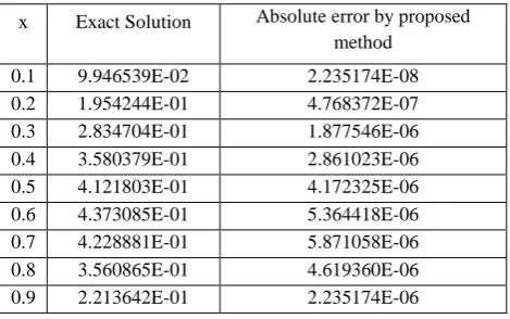
[image:3.595.312.547.459.606.2]The exact solution for the above problem is given by y(x) = x(1-x)ex. The proposed method is tested on this problem where the domain [0,1] is divided into 10 equal subintervals. Numerical results for this problem are shown in Table 1. The maximum absolute error obtained by the proposed method is 5.871058 × 10⁻⁶.
Table 1. Numerical results for Example 1
x Exact Solution Absolute error by proposed method
0.1 9.946539E-02 2.235174E-08 0.2 1.954244E-01 4.768372E-07 0.3 2.834704E-01 1.877546E-06 0.4 3.580379E-01 2.861023E-06 0.5 4.121803E-01 4.172325E-06 0.6 4.373085E-01 5.364418E-06 0.7 4.228881E-01 5.871058E-06 0.8 3.560865E-01 4.619360E-06 0.9 2.213642E-01 2.235174E-06
Example 2 Consider the linear boundary value problem y(5) - y(4) = -ex (2x +7), 0 < x < 1 (19) subject to the boundary conditions
y(0) = 0, y(1) = 0, y’(0) = 1, y’(1) = -e, y’’(0) = 0.
Table 2. Numerical results for Example 2
x Exact Solution Absolute error by proposed method 0.1 9.946539E-02 6.705523E-08
0.2 1.954244E-01 7.748604E-07 0.3 2.834704E-01 2.682209E-06 0.4 3.580379E-01 4.351139E-06 0.5 4.121803E-01 6.288290E-06 0.6 4.373085E-01 7.808208E-06 0.7 4.228881E-01 8.165836E-06 0.8 3.560865E-01 6.347895E-06 0.9 2.213642E-01 2.950430E-06
Example 3 Consider the linear boundary value problem
y(5)(x) + y(4)(x) + e-2x y(x) = e-x[–4e2x(–3 + x) cosx – {1 – x + 4e2x
(5+2x)}sinx], 0 < x <1 (20) subject to the boundary conditions
y(0) = 0, y(1) = 0, y’(0) = -1, y’(1) = e sin1, y’’(0) = 0.
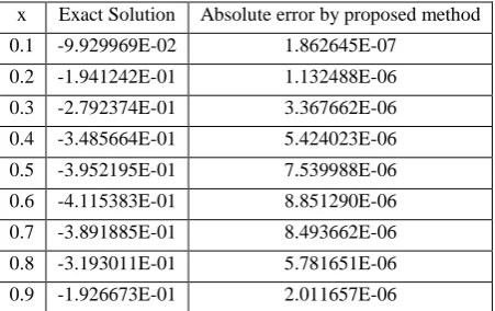
The exact solution for the above problem is given by y(x) = ex(x –1)sinx. The proposed method is tested on this problem where the domain [0,1] is divided into 10 equal subintervals. Numerical results for this problem are shown in Table 3. The maximum absolute error obtained by the proposed method is 8.851290 × 10⁻⁶.
Table 3. Numerical results for Example 3
x Exact Solution Absolute error by proposed method 0.1 -9.929969E-02 1.862645E-07
0.2 -1.941242E-01 1.132488E-06 0.3 -2.792374E-01 3.367662E-06 0.4 -3.485664E-01 5.424023E-06 0.5 -3.952195E-01 7.539988E-06 0.6 -4.115383E-01 8.851290E-06 0.7 -3.891885E-01 8.493662E-06 0.8 -3.193011E-01 5.781651E-06 0.9 -1.926673E-01 2.011657E-06
Example 4 Consider the linear boundary value problem y(5)(x) + (x–2) y(4)(x) + 2y’’’(x) – (x2+2x–1)y’’(x)
+(2x2+4x)y’(x) – 2x2y(x) = 4excosx – 2x4 + 4x3 + 6x2 – 4x + 2,
0 < x <1 (21)
subject to the boundary conditions
y(0) = 0, y(1) = 1+2e sin1, y’(0) = 2, y’(1) = 2e(sin1+cos1)+2, y’’(0) = 6.
The exact solution for the above problem is given by y(x) = 2exsinx+x2. The proposed method is tested on this problem where the domain [0,1] is divided into 10 equal subintervals. Numerical results for this problem are shown in Table 4. The
[image:4.595.317.544.125.271.2]maximum absolute error obtained by the proposed method is 2.670288× 10⁻⁵.
Table 4. Numerical results for Example 4
x Exact Solution Absolute error by proposed method 0.1 2.306660E-01 4.619360E-07
0.2 5.253106E-01 2.384186E-06 0.3 8.878211E-01 7.808208E-06
0.4 1.321888 1.180172E-05
0.5 1.830878 1.740456E-05
0.6 2.417691 2.288818E-05
0.7 3.084590 2.670288E-05
0.8 3.833011 1.764297E-05
0.9 4.663347 8.106232E-06
Example 5 Consider the nonlinear boundary value problem y(5) = ex[y(x)]4, 0<x<1 (22) subject to the boundary conditions
. 9 1 ) 0 (
, 3 1 ) 1 ( , 3 1 ) 0 (
, ) 1 ( , 1 ) 0 (
''
3 1 '
'
3 1
y
e y
y
e y y
This nonlinear boundary value problem is converted into a sequence of linear boundary value problems generated by quasi linearization technique [17] as
y(5)(n+1)(x) - [4e x
y3(n)]y(n+1) = -3e x
y4(n), n = 0,1,2,… (23)
subject to the boundary conditions
.
9
1
)
0
(
,
3
1
)
1
(
,
3
1
)
0
(
,
)
1
(
,
1
)
0
(
) 1 ( ''
3 1
) 1 ( ' )
1 ( '
3 1
) 1 ( )
1 (
n
n n
n n
y
e
y
y
e
y
y
[image:4.595.55.281.445.587.2]Table 5 Numerical results for Example 5
x Numerical solutions obtained by Hussin and Kilicman [22]
Absolute error by the proposed method when compared with
Hussin and Kilicman [22]
0.1 9.672161E-01 8.344650E-07
0.2 9.355070E-01 2.622604E-06
0.3 9.048374E-01 5.960464E-06
0.4 8.751733E-01 7.510185E-06
0.5 8.464817E-01 8.881092E-06
0.6 8.187308E-01 9.298325E-06
0.7 7.918895E-01 8.404255E-06
0.8 7.659283E-01 5.125999E-06
0.9 7.408182E-01 2.026558E-06
Example 6 Consider the nonlinear boundary value problem
εy’ y(5)
+ y(4) = –120x + 600ε(x2–1/4)(x2–1/20), –1/2<x<1/2 (24) subject to the boundary conditions
. 1 ) 2 / 1 (
, 0 ) 2 / 1 ( , 0 ) 2 / 1 (
, 0 ) 2 / 1 ( , 0 ) 2 / 1 (
''
' '
y
y y
y y
The exact solution is y = -x(x2-1/4)2.. This nonlinear boundary value problem is converted into a sequence of linear boundary value problems generated by quasi linearization technique [17] as
[εy’
(n)]y(5)(n-+1) + y(4)(n-+1)+[εy(5)(n)]y’(n+1) = –120x + 600ε(x2–1/4)(x2–1/20) + εy’(n) y
(5) (n)
for n = 0,1,2,… (25)
subject to the boundary conditions
. 1 ) 2 / 1 (
, 0 ) 2 / 1 ( , 0 ) 2 / 1 (
, 0 ) 2 / 1 ( , 0 ) 2 / 1 (
1 ''
1 ' 1
'
1 )
1 (
n
n n
n n
y
y y
y y
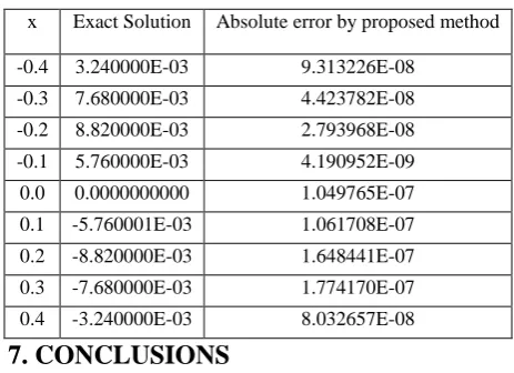
[image:5.595.312.544.86.254.2]Here y(n+1) is the (n+1)th approximation for y. The domain [-1/2, 1/2] is divided into 10 equal subintervals and the proposed method is applied to the sequence of problems (25). Numerical results for this problem with ε = 0.01 are presented in Table 6. The maximum absolute error obtained by the proposed method is 1.774170× 10⁻⁷.
Table 6. Numerical results for Example 6
x Exact Solution Absolute error by proposed method
-0.4 3.240000E-03 9.313226E-08 -0.3 7.680000E-03 4.423782E-08 -0.2 8.820000E-03 2.793968E-08 -0.1 5.760000E-03 4.190952E-09 0.0 0.0000000000 1.049765E-07 0.1 -5.760001E-03 1.061708E-07 0.2 -8.820000E-03 1.648441E-07 0.3 -7.680000E-03 1.774170E-07 0.4 -3.240000E-03 8.032657E-08
7. CONCLUSIONS
In this paper, we have developed a collocation method with quartic B-splines as basis functions to solve fifth order boundary value problems. Here we have taken internal mesh points x1, x2, …, xn-1 as the selected collocation points. The quartic B-spline basis set has been redefined into a new set of basis functions which in number match with the number of selected collocation points. The proposed method is applied to solve several number of linear and non-linear problems to test the efficiency of the method. The numerical results obtained by the proposed method are in good agreement with the exact solutions available in the literature. The objective of this paper is to present a simple method to solve a fifth order boundary value problem and its easiness for implementation.
8.
REFERENCES
[1] Davies. A.R, Karageorghis. A, Phillips. T.N. “Spectral Galerkin methods for the primary two point boundary-value problems in modelling viscoelastic flows”. Internat. J. Numer. Methods Engrg. 16 (1988): 647-662. [2] Karageoghis. A, Phillips. T.N, Davies. A.R. “Spectral
collocation methods for the primary two-point boundary-value problems in modelling viscoelastic flows”. Internat. J. Numer. Methods Engg. 26 (1998): 805-813. [3] Agarwal. R.P, 1986, Boundary Value Problems for
Higher Order Differential Equations, World Scientific, Singapore.
[4] Caglar. H.N, Caglar. S.H, Twizell. E.H. “The numerical solution of fifth order boundary-value problems with sixth degree B-spline functions”. Appl. Math. Lett. 12 (1999): 25-30.
[5] Siddiqi. S.S, Akram. G. “Sextic Spline Solution of fifth order boundary value problems”. Applied Mathematics Letters 20 (2007): 591-597.
[6] Lamini. A, Mraoui. H, Sbibih. D, Tijini. A. “Sextic Spline Solution of fifth order boundary value problems”. Mathematics and Computers in Simulation 77(2008): 237-246.
[8] Wazwaz. A.M. “The numerical solution of fifth-order boundary value problems by the decomposition method”. J. Comput. Appl. Math. 136(2001) : 259-270.
[9] Khan. M.A, Siraj-ul-Islam. I.A, Tirmizi. E.H, Twizell. S. Ashraf. “A class of methods based on non-polynomial sextic spline functions for the solution of a special fifth-order boundary-value problems”. J. Math. Anal. Appl. 321(2006) : 651-660.
[10] El-Gamel. M. “Sinc and the numerical solution of fifth-order boundary value problems”. Appl. Math. Comput. 187(2007): 1417-1433.
[11] Noor. M.A, Mohyud-Din. S.T. “An effcient algorithm for solving fifth order boundary value problems”. Math. Comput. Modelling. 45(2007): 954-964.
[12] Kasi Viswanadham. K.N.S., Murali Krishna. P, Prabhakara Rao. C. “Numerical Solution of Fifth Order Boundary Value Problems by Collocation Method with Sixth Order B-splines”. Internatinal Journal of Applied Science and Engineering, 8(2010): 119-125.
[13] Kasi Viswanadham. K.N.S., Murali Krishna. P. “Quintic B-splines Galerkin Method for Fifth Order Boundary Value Problems”. ARPN Journal of Engineering and Applied Sciences, 5(2010): 74-77.
[14] Fyfe. D.J. “Linear dependence relations connecting equal interval Nth degree splines and their derivatives”. J. Inst. Math. Appl. 7(1971): 398-406.
[15] Zhao-ChunWu. “Approximate analytical solutions of fifth-order boundary value problems by the variational iteration method”. Computers and Mathematics with Applications 58 (2009): 2514-2517.
[16] Juan Zhang. “The numerical solution of fifth-order boundary value problems by the variational iteration method”. Computers and Mathematics with Applications 58 (2009): 2347-2350.
[17] Bellman. R.E, Kalaba R.E., 1965, Qusilinearization and Nonlinear Boundary value problems. American Elsevier, New York.
[18] Reddy. J.N., 2005, An introduction to the Finite Element Method, Tata Mc-GrawHill Publishing Company Limited, 3rd Edition, New Delhi.
[19] Prenter. P.M., 1989, Splines and Variational Methods, John-Wiley and Sons, New York.
[20] Carl de Boor, 1978, A Practical Guide to Splines, Springer-Verlag.
[21] Schoenberg. I.J., 1966, On Spline Functions, MRC Report 625, University of Wisconsin.