Sharif University of Technology
Scientia IranicaTransactions B: Mechanical Engineering http://scientiairanica.sharif.edu
A modied wavelet energy rate-based damage
identication method for steel bridges
M. Noori
a, H. Wang
b, W.A. Altabey
c;, and A.I.H. Silik
da. International Institute for Urban Systems Engineering, Southeast University, Nanjing 210096, China; and Mechanical Engineering and ASME Fellow, California Polytechnic State University, San Luis Obispo, California, USA.
b. State University of New York, Bualo, NY 14260, USA.
c. International Institute for Urban Systems Engineering, Southeast University, Nanjing 210096, China, Nanjing Zhixing Information Technology Company Nanjing; China; and Department of Mechanical Engineering, Faculty of Engineering, Alexandria University, Alexandria 21544, Egypt.
d. International Institute for Urban Systems Engineering, Southeast University, Nanjing 210096, China. Received 12 March 2018; accepted 2 July 2018
KEYWORDS FBG strain sensor; Wavelet packet transform;
Damage identication; Modied wavelet packet energy rate.
Abstract. Strain is sensitive to damage, especially in steel structures. However, a traditional strain gauge does not t bridge damage identication because it only provides the strain information of the point, where it is set up. While traditional strain gauges suer from drawbacks, a long-gage FBG strain sensor is capable of providing the strain information of a certain range, in which all the damage information within the sensing range can be reected by the strain information provided by FBG sensors. The wavelet transform is a new way to analyze the signals, capable of providing multiple levels of details and approximations of the signal. In this paper, a wavelet packet transform-based damage identication is proposed to identify the steel bridge damage numerically and with experimentally to validate the proposed method. The strain data obtained via long-gage FBG strain sensors are transformed into a modied wavelet packet energy rate index rst to identify the location and severity of damage. The results of numerical simulations show that the proposed damage index is a good candidate that is capable of identifying both the location and severity of damage under noise eect.
© 2018 Sharif University of Technology. All rights reserved.
1. Introduction
Since steel bridges suer from complex working con-ditions during their service life, heavy working loads and other eects damage structures and accelerate the development of damages. With the accumulation of damages to structures, the safety of both the structure and human life can be threatened and may directly
*. Corresponding author. Tel.: +86-17368476644 E-mail addresses: [email protected] (M. Noori); [email protected] (H. Wang); [email protected] (W.A. Altabey); [email protected] (A.I.H. Silik)
doi: 10.24200/sci.2018.20736
result in tragedies of life and property [1,2]. There-fore, structural damage identication has become an important research topic in the engineering protection eld [3]. Over the last two decades, the consider-able development of integrated monitoring systems for new and existing structures worldwide, such as steel bridges, has been recognized as an important tool to solve structural damage identication problem. It is commonly stated in the structural health monitoring literature that damage identication approaches are classied as methods based on time domain analysis [4], methods based on modal parameters [5], and methods based on time-frequency domain analysis [6]. The majority of these techniques are based on vibration that require data acquisition instruments to be xed
on the bridge directly, which may be dicult and time-consuming; however, it is eective in giving a warning to people if there is any indication of hazard on Bridge's condition. These methods become a more important part of bridge monitoring systems.
In recent years, there have been movement to-wards the development of indirect vibration methods based on a vehicle response moving over a bridge. These methods aimed to reduce the need of installing instruments directly on bridge to achieve more e-ciency and low cost. In related development, Bu et al. [7] and McGetrick & Kim [8] investigated numer-ically a bridge condition using the dynamic response of a vehicle running along a beam to evaluate related damage based on reduction of stiness. The results showed that vehicle speed, road surface roughness, measurement noise, and numerical model errors did not have signicant eect on the accuracy of the method. In addition, Gonzalez et al. [9] innovated a novel algorithm using the vehicle acceleration as an algorithm input to determine the damping of a bridge. It was shown that the algorithm could be used for bridge stiness identication. It was also stated that the algorithm was not highly sensitive to signal with low-level noise, the road roughness, and model errors.
Furthermore, current damage detection tech-niques can be classied into two broad categories: local and global damage identications. Most global damage identication methods rely on damage-induced changes in the dynamic properties of the identied structure. In these identication methods, system parameters, such as frequencies, deected mode shapes, strain energy, exibility matrix, etc., are used as part of the damage index [10]. Among the discussed damage detection methods, some are directly based on Fourier transform (e.g., natural frequency-based damage identication methods). Fourier transform provides information in the frequency domain and is not capable of detecting when (or where) a particular damage occurs. To overcome this disadvantage, Dennis Gabor proposed the Short-Time Fourier Transform (STFT). This well-known windowing technique divides the signals into a series of sections. Each time, STFT is done within a small window that represents a section of the signal. Thus, information on both frequency and time domains can be kept. However, STFT has a disadvantage: the information about time and frequency (or space and frequency) is acquired with limited precision. According to the Heisenberg uncertainty theory, this limitation is determined by the size of the time-frequency window. Once the window size is set, it is the same for all frequencies; therefore, a higher resolution in time and frequency domains (or space and frequency domain) cannot be acquired simultaneously.
The Wavelet Transform (WT) is a relatively new signal-processing tool to analyze data. Based on the
theory of WT, it can be viewed as an extension of traditional STFT transform with adjustable window location and size. With its unique merit of examining signals with a \zoom lens having an adjustable focus", the original signal is separated into two dierent levels of details and approximations [11-13]. Therefore, transient information of the signal can be retained. The wavelet transform as a technique for structural damage identication has been introduced recently due to its capability of capturing the transient behavior of a signal and analyzing it in time and frequency domains, as investigated by several researchers. Hester et al. [14] demonstrated the ability of the wavelet transform to get information from time-frequency domains, while Zhao et al. [15-17] employed the structural mode shapes that extracted from the nite element model of a simply supported reinforced concrete beam for damage identication using dierent types of wavelets. Reda Taha et al. [18] discussed in detail various aspects re-lated to wavelet transform as a technique for structural damage. Nguyen and Tran [19] provided a method based on Symlet wavelet to evaluate bridge cracks from vehicle displacement response. It was concluded that cracks can be detected; however, higher speeds give poor detection than low speed. Lee et al. [20] provided an algorithm for truss bridge based on the continuous relative wavelet entropy. It was concluded that damage could be detected; however, computation cost is very large for the real-life monitoring. Although signicant research has been carried out in the area of structural health monitoring to make structures work safely, highly reliable and practical damage identica-tion methods are still lacking and many disasters occur due to lack of damage identication.
Strain measurements have proved to be sensitive to damage. However, if traditional strain gauges are not installed exactly on the damaged locations, the damage detection result will not be accurate. Thus, the idea of distributed sensing system was proposed to overcome the limitation of the traditional strain gauge in obtaining the strain, where they are installed [21]. Distributed sensing system is dierent from multipoint sensing system. It is capable of capturing the informa-tion within a certain range of the structure, leading to integrated information of the entire structure.
However, this requirement of distributed sensing systems was unreachable until Horiguchi et al. [22] proposed the relationship between the strain and Bril-louin frequency shift in optical bers. Based on this relationship, a concept of distributed sensing system was proposed. Subsequently, Fiber Bragg Grating (FBG) sensors [23], Brillouin Optical Time Domain Reectometer (BOTDR) sensors [24,25], and Brillouin Optical Time Domain Analysis (BOTDA) have been widely used in long-gage strain monitoring systems.
wavelength of the reective signal from the grating changes when it has longitudinal deformation. By mea-suring the changes of wavelength, accurate deformation of the grating can be achieved. Based on wavelength-division multiplexing technology, several FBG sensors can be combined in one ber to achieve multipoint sensing. For long-gage FBG sensors [26], ber Bragg gratings are packaged in series to extend the eective sensing length. FBG sensors have their own merit: the signals used in FBG sensors are wavelength-modulated signals, meaning that they do not need to suer from the limitations of inaccurate phase measurement used in other kinds of ber optic sensors.
BOTDR and BOTDA sensors are based on Bril-louin scattering [24,25]. Once there is a change in strain or temperature on the ber, the central fre-quency of Brillouin scattering light changes. Based on the relationship, Brillouin scattering light can be used to acquire changes in strain and temperature. For BOTDR and BOTDA sensors, any part of the ber is both a sensing unit and a signal transmission unit, leading to their capability of spatial continuous measurement.
BOTDR/BOTDA sensors and FBG sensors have dierent merits based on their sensing concept. FBG sensors have better accuracy in both dynamic and static sensing. However, theoretically, FBG sensors are point sensors. Their sensing length is limited. The ac-curacy and sampling rate of BOTDR/BOTDA sensors is lower than those of FBG sensors. However, they are more suitable for distributed sensing, especially in large-scale structures. With the consideration of the small scale of the laboratory, long-gage FBG sensors are adopted in this research.
In this paper, the goal is to investigate the eectiveness of a modied wavelet energy rate-based damage identication method for steel bridges elements (beam and frame). Both simulated and experimen-tal experiments are utilized to validate the proposed method. Measured dynamic signals from structures are rst decomposed into the wavelet packet components. Then, the modied wavelet packet strain energy rate index is calculated based on the wavelet packet compo-nents and is, then, used to locate the damage and assess the severity of damage. Dierent scenarios are con-sidered to validate the proposed damage identication method. The simulated test results show that the pro-posed damage identication method is able to detect both location and severity of damages to a structure. 2. Theoretical background
2.1. Wavelet and continuous wavelet transform
Wavelet analysis is a signal processing method that relies on the introduction of an appropriate basis and
characterization of the signal by the distribution of amplitude on the basis [27]. If the wavelet is required to form a proper orthogonal basis, it has the advantage that an arbitrary function can be uniquely decomposed, and the decomposition can be inverted. The wavelet is a smooth and quickly vanishing oscillating function with good localization in both frequency and time. A wavelet family, a;b(t), is a set of elementary functions
generated by dilations and translations of a unique admissible mother wavelet, (t):
a;b(t) = p1a
t b
a
; (1)
where b 2 R, a > 0 are the scale and translation parameters, respectively, and t is time (or location, if wavelet transform is utilized in spatial distributed signal). As scale parameter a increases, the wavelet becomes wider. Therefore, each parameter shows the signal at dierent scales and with variable time (or space localization).
The wavelet transform (in its continuous or dis-crete version) correlates function f(t) with a;b(t). The
Continuous Wavelet Transform (CWT) is the sum of all time of the signal multiplied by a scaled and shifted version of a mother wavelet:
C (a; b) =p1 a 1 Z 1 f (t) t b a dt: (2)
The results of the transform are wavelet coe-cients, determining how the wavelet function signal expresses the signal. Hence, sharp transitions f(t) create wavelet coecients with large amplitudes, and this precisely is the basis of the proposed damage identication method.
The CWT has an inverse: The inverse CWT helps to recover the signal from its coecients C(a; b) and is dened as follows:
f (t) = 1 K +1 Z a +1 Z 1
C (a; b) a;b
t b
a
1
a2dadt; (3)
where constant K is: K =
+1
Z
0
^ (!)2
b!c d!: (4)
2.2. Discrete Wavelet Transform (DWT) and Wavelet Packet Transform (WPT)
There is still a drawback to the CWT: A very large number of wavelet coecients C(a; b) are generated during the analysis [28]. It can be shown that the CWT is highly redundant, because it is not necessary
to use the full domain of C(a; b) to reconstruct f(t). Therefore, instead of using a continuum of dilations and translations, discrete values of the parameters are used in Discrete Wavelet Transform (DWT). The dilation is dened as a = 2j, and the translation parameter
takes the values of b = k2j, (j; k) 2 Z, and Z is a set
of integers. It has been proved that DWT can fully decompose a signal without losing any part of it. This sampling of the coordinates is referred to as dyadic sampling, because consecutive values of the discrete scales dier by a factor of 2 [29]. Using the discrete scales, one can dene the DWT:
Cj;k= 2 j2
Z +1
1 f(x) 2
jx kdx
= Z +1
1 f(x) j;k(x)dx: (5)
The signal resolution is dened as the inverse of the scale 1=a = 2 j, and integer j is referred to
as the level. As the decomposition level increases, the frequency resolution increases, and the smaller bandwidth components of the signal can be obtained.
The signal can be reconstructed from wavelet coecients, Cj;k, and the reconstruction algorithm is
called the Inverse Discrete Wavelet Transform (IDWT): f(x) = X1
j= 1 1
X
k= 1
Cj;k2 j=2 (2 jx k): (6)
One possible drawback to the DWT is that the frequency resolution is quite poor in the high-frequency region. It is dicult for DWT to discriminate signals containing close high-frequency components. The Wavelet Packet Transform (WPT) is one extension of the DWT that provides complete level-by-level decomposition. The wavelet packets are alternative bases formed by linear combinations of the usual wavelet functions. The decomposed subcomponents can be treated as narrow-band signals under high decomposition levels.
Wavelet packets consist of a set of linearly com-bined usual wavelet functions. The wavelet pack-ets inherit properties, such as orthonormality and time-frequency localization, from their corresponding wavelet functions [30]. A wavelet packet is a function with three indices, i
j;k(t) where integers i, j and
k are the modulation, the scale, and the translation parameter, respectively.
i
j;k(t) = 2j=2 i(2jt k); i = 1; 2; :::: (7)
The wavelets, i, are obtained from the following
recursive relationships:
2i(t) =p2 X1 k= 1
h(k) i(2t k); (8)
2i+1(t) =p2 X1 k= 1
g(k) i(2t k): (9)
The rst wavelet is the so-called mother wavelet func-tion:
1(t) = (t): (10)
Discrete lters h(k) and g(k) are quadrature mirror lters associated with the scaling function and the mother wavelet function, which can be treated as low-pass and high-pass lters. A quadrature mirror lter is a lter whose magnitude response is the mirror image around =2 of that of another lter. There are quite a few mother wavelets reported in the literature. Most of these mother wavelets are developed to satisfy some important properties, such as the invertibility and the orthogonality. Daubechies developed a family of mother wavelets based on the solution of a dilation equation. One of these wavelets, DB20, is adopted in this study.
Similar to the FT, any measurable and square-integrable function can be decomposed into wavelet packets. The decomposition process is a recursive lter-decimation operation. Figure 1 shows a full WPT tree
of a time-domain signal, f(t), up to the 3rd level of decomposition. Figure 1 shows that the DWT consists of one high-frequency term from each level and one low-frequency residual from the last level of decomposition. The WPT, on the other hand, contains complete decomposition at every level and, hence, can achieve a higher resolution in the high-frequency region. The recursive relations between the jth and the j +1th level components are:
fi
j(t = f(j+1)(2i 1)(t) + f(j+1)2i (t); (11)
fj+12i 1(t) = Hfi
j(t); (12)
f2i
j+1(t) = Gfji(t); (13)
where H and G are ltering-decimation operators and are related to discrete lters, h(k) and g(k), through:
H (t) = X1
k= 1
h (k 2t); (14)
G (t) = X1
k= 1
g (k 2t): (15)
After j levels of decomposition, original signal f(t) can be expressed as follows:
f(t) = 2
j
X
i=1
fi
j(t): (16)
The wavelet packet component signal, fi
j(t), can be
expressed by a linear combination of wavelet packet functions, i
j;k(t), as follows:
fi j(t) =
1
X
k= 1
ci
j;k j;ki (t): (17)
The wavelet packet coecients, ci
j;k, can be obtained
from: ci j;k= Z +1 1 f(t) i
j;k(t)dt: (18)
Providing that the wavelet packet functions are orthog-onal:
m
j;k(t) nj;k(t) = 0; if m 6= n: (19)
Each component in the WPT tree can be viewed as the output of a lter tuned to a particular basis function; thus, the whole tree can be regarded as a lter bank. At the top of the WPT tree (lower level), the WPT yields good resolution in the time domain, yet poor resolution in the frequency domain. At the bottom of the WPT tree (higher level), the WPT results in good resolution in the frequency domain, yet poor resolution in the time domain.
2.3. Modied wavelet packet energy rate 2.3.1. The Continuous Wavelet Transform (CWT)
wavelet packet energy
Energy concentration is one of the reliable features of time-frequency data processing. Particularly, energy has been used successfully for classication application. Thus, the wavelet packet energy representation can provide more robust signal features for classication, while it is dicult to identify these features directly from the expansion coecients [31,32]. Furthermore, wavelet packet energy can be used to identify the locations and severity of damage. To do that, wavelet packet energy, Enj, at j level of node n is dened as
follows: Enj =
Z +1
1 f
2(t)dt = 2
j X m=1 2j X n=1 Z +1 1 f m
j (t)fjn(t)dt
=
2j
X
i=1
Eni
j: (20)
A signal f(t) should be square integrable if En is
nite, that is, f(t) is in Hilbert space L2(R).
Note that energy in this context is not the same as the conventional notion of energy in other areas of science. The signal energy at the jth level and the ith frequency band can be expressed as follows:
Ej= n
X
k=1
jCj(k)j2; j = 1; 2; : : : : : : ; m: (21)
The total energy of signal is expressed by: Efj =
2j
X
i=1
Efi
j
; (22)
where wavelet packet component energy, Eni
j, can be
considered to be the energy stored in component signal, fi
j(t):
Eni
j =
Z +1
1 f i
j(t)2dt: (23)
Eq. (20) demonstrates that the overall signal energy can be spilt to wavelet packet energy components in various, frequency bands. Finally, the WPERI was developed to identify the location and extent of the damage of the crack [33]:
Efj
= 2j X i=1 Efi
j
b
Efi
j a
Efi j
a
: (24)
The term (Efi
j)a is the signal component energy
at level j without damage, and (Efi
j)b is the signal
is assumed that structural damage can inuence the wavelet packet component energies and, then, may change this damage indicator. Therefore, it is desired to choose the Wavelet Packet Energy Rate Index (WPERI), because it is sensitive to the alerts in the signal characteristics [34].
2.3.2. Modied wavelet packet energy
Structural damage detection utilizing wavelet packet energy is one of the most reliable and ecient struc-tural health monitoring techniques. The energy meth-ods, which are based on strain response data, are rather sensitive compared to those based on acceleration and displacement, because strain energy density involves the second spatial derivatives of the displacement; in addition, it is much more sensitive to small deviation in the structural response than to the displacement itself. Therefore, wavelet packet energy has been modied to include the eect of strain in order to increase the accuracy of damage detection. It is expected that de-ploying the modied method can obtain more accurate strain energy stored in structural elements; at the end, it provides appropriate, damage detection model and reduces the computation and iteration eorts.
Strain is rather more sensitive to damage than to other raw data, such as deection, velocity, and acceleration. In certain cases, damage can be directly identied via raw strain data. For structural dynamic responses, the Envelope Area of Strain-time Curvature (EASC) is proposed as a damage index:
Sn=
Z +1
1 fn(t)dt: (25)
To quantify the damage from wavelet packet com-ponent energies, the Modied Wavelet Packet Energy Rate (MWPER) is proposed in this paper to detect both the location and severity of the damage. MWPER of node n is dened as follows:
Dn = 2j
X
i
(Eni
j)a (Enij)b
[(Sn)a (Sn)b]
; (26) where subscripts a and b stand for damaged and undamaged statuses, respectively.
Wavelet packet energy rate is capable of utilizing information extracted from dierent frequency-bands, and the envelope area of strain-time curvature extracts the amplitude information from strain time-history data. Thus, MWPER can utilize both the frequency domain information and amplitude information of the raw data.
For a damage identication procedure based on the modied method, it is assumed that the reliable intact and damaged structural models are available, and the structure is excited via the same impulse load and acts at the same location in damage and undamaged structures.
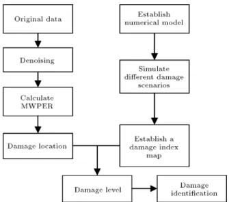
Figure 2. Flow chart of damage identication based on strain-time history data.
3. Damage identication procedure
Based on the discussion above, a complete damage identication procedure is established for the second method. Figure 2 shows the complete procedure of damage identication based on WT. The steps for this procedure are described below.
3.1. Establishment of a numerical model Developing a numerical model is the rst step to detect the severity of the damage. Thus, a ne mesh numerical model of the structure should be established.
3.2. Simulation of running car experiments At least, four points of damage need to be simulated as described below:
(a) Damage at point DB1 with stiness loss of SL1;
(b) Damage at point DB1 with stiness loss of SL2;
(c) Damage at point DB2 with stiness loss of SL1;
(d) Damage at point DB3 with stiness loss of SL1. Based on the MWPER data from simulations (a) and (b) above, the near-linear relationship between the stiness loss and MWPER can be determined. Based on the MPWER data of (a), (c), and (d), the relationship between the location and MPWER at (a) certain level of damage severity can be determined. 3.3. Establishment of the damage index map Based on the relationships obtained in the previous section, a damage index map is established.
3.4. Denoising of the input signal
The original data used in this research represent long-gauge strain data obtained via FBG/BOTDR sensors. As discussed before, denoising is commonly the rst step for signal processing. Then, all input signals will be denoised by WT.
3.5. Calculation of MWPER
Based on the value of MPWER, the damage location can be found.
3.6. Combination of the damage location and the value of MWPER
Since a map is developed where all the relationships have been established, the severity of the damage can be determined by examining the corresponding location and the data from MPWER.
3.7. Maintenance decision based on the damage location information
Once the damage location and its severity are veried, it can be determined if the structure needs to be repaired.
4. Validation by numerical models
A completed theory for damage identication scheme needs to be validated by experiments. Thus, numerical simulations are essential for the development of the proposed method. The theoretical background has been elaborated in the previous section; hence, numer-ical simulations are introduced herein to validate this method.
4.1. Numerical model
In this section, MWPER is introduced as a damage index, whose calculation is based on WPER and EASC, and the calculation of wavelet packet energy is based on strain time history data of the structure. Since the entire damage identication is based on the strain-time history data, the model used in this section should be able to have enough strain at every part of the structure. Although a simply supported beam will not have any strain at the support points, the supporting condition of xed ends and simply supported beams can both be considered and compared to see if the proposed method identies damages in the vicinity of the supports of a simply supported beam. In this work, both beam and single-layer frame models will be used to validate the proposed damage identica-tion.
ANSYS 14.5 is introduced as a numerical simula-tion platform. For the convenience of modeling, all the material properties and cross-sections are set to be the same among all models. The material properties used herein have been commonly used in numerous research works, including: E = 200 GPa, = 7800 kg/m3, and
= 0:3, where E stands for Yong's modulus, stands for mass density, and stands for Poisson's ratio.
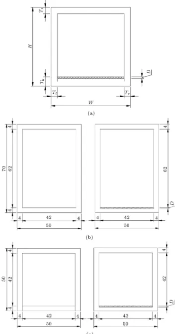
All three numerical models are described in detail below. For the convenience of comparison and mod-eling, undamaged and damaged sections of beams and columns in all 3 models are set to be the same. A total of 8 section scenarios are considered in this paper
Figure 3. Sections of undamaged and damaged columns and beams: (a) The section used for the calculation of bending rigidity, (b) sections of undamaged and damaged beam, and (c) sections of undamaged and damaged column.
for the beam model. The beam section is set to be a thin-walled rectangular tube, whose height, width, and thickness are 70 mm, 50 mm, and 4 mm, respectively (Figure 3(a)). The column section is set to be a square steel tube, whose height, width, and thickness are 50 mm, 50 mm, and 4 mm, respectively (Figure 3(b) and (c)). Corrosion or crack on bridges reduces the working area of the component sections; thus, the damage is simulated by reducing wall thickness. Since hydrops cause corrosion at the bottom wall of a structure, the thickness of bottom wall will be reduced so as to simulate damages. The reduced part of the
bottom walls is shown in Figure 3(a), (b), and (c) as the shaded parts.
All damages/cracks are simulated by reducing the thickness of the bottom layer. The stiness loss should be calculated exactly, since the wavelet coecients might be used as a damage index that are able to reect the damage severity. For the purpose of simulating the damages with dierent damage levels, a formula is proposed to calculate the exact thickness loss that is needed for a certain bending rigidity loss. The second moment of area is:
I =Tt123W + TtW
Hn T2t
2
+(Tb 2d)3W
+ W (Tb d)
H Hn Tb2 d
2
+Tl(H Tt12 Tb+ d)3
+ Tl(H Tt Tb+ d)
(H Tt Tb+ d)
2 + Tt Hn 2
+Tr(H Tt12 Tb+ d)3
+ Tr(H Tt Tb+ d)
(H Tt Tb+ d)
2 + Tt Hn 2
: (27)
Hn and all the parameters, such as W , H, d, Tt, Tb, Tl
and Tr, are shown in Figure 3(b) and (c), where:
Hn =
W H2
2
(H+d) (H +d Tt Tb) (W Tl Tr)
2
[W H (W Tl Tr) (H + d Tt Tb)]:
With this formula, a damage ranging from zero to 30% bending rigidity loss is proposed for the following sections. Table 1 shows the exact thickness loss of the bottom layer.
Table 1 shows all beam section information listed in column sections; only one damage severity level is used, and the stiness loss of that damage is 3.81%.
D represents the section plots (Figure 3(b) and (c)) which stand for damage depths; for the con-venience of description, zero damage depth means that there is no damage at the corresponding section (Section ID 1 as described in Table 1).
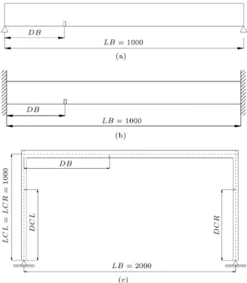
The damage location information for the adopted numerical models introduces the following detail:
Model 1: Simply supported beam. The simply supported beam's length is set to be 1000 mm, with a damage introduced at distances of DB from the left support as shown in Figure 4(a).
Model 2: Fixed ends beam. The xed ends beam's length is set to be 1000 mm, which is the same as the simply supported beam's. The damage location parameter, DB, is dened as the distance
Figure 4. Detail of The numerical models: (a) Simply supported beam model, (b) xed ends beam model, and (c) single layer frame model.
Table 1. Section information of all the sections used in this work.
Section type Beam section
Section ID 1 2 3 4 5 6 7 8
Area (mm2) 896 875 867 840 816 794 774 755
Damage depth (mm) 0 0.5 0.6972 1.3252 1.8964 2.4202 2.9037 3.3525 IY (10E6 mm4) 5.95 5.74 5.65 5.36 5.06 4.76 4.46 4.17
between the damage location and the left support, as shown in Figure 4(b).
Model 3: Single layer frame. The single layer frame shown in Figure 4(c) is used as the 3rd numerical model. Damages are marked by rectangular symbols in Figure 4(c), and DB is the distance of the damage location from the centroidal axis of the left column. LB is the total length of the beam. DCL is the distance from the centroidal axis of the left column, while LCL is the total length of the column. The unit used in Figure 4(c) is mm. 5. Damage scenarios
To establish the second method, several dierent dam-age scenarios need to be taken into consideration. There are three cases for the establishment and vali-dation of that method.
Firstly, two dierent kinds of excitations are compared, simulated via contact elements in ANSYS. So far, most dynamic experiments are done by hammer excitation. For bridges, cars run on the top of the beam. Both running car excitations and hammer excitations are usually used for dynamic experiments on bridges; thus, these two types of excitations are adopted in this work. The hammer is simulated by 8 kg mass, and it hits the structure at a speed of 4 m/s. The running car is simulated by 8 kg mass and the car runs from the left side to the right side at a speed of 2 m/s. Secondly, the situation in which damages occur at points where the strain is relatively small must be taken into consideration to validate if the proposed method can be used independently to detect without additional detection method. As mentioned in the previous sections, the proposed method only works in the context in which strain exists in every part of the structure. For steel bridges, although stain exists everywhere on the structure, there are always some points where the strain is relatively small, making it essential to validate the proposed method for small-strain situation cases.
Thirdly, a multiple-damage scenario must be taken into consideration, since the damages/cracks on steel bridges may occur simultaneously. Although the theory behind the second damage identication method indicates that the spatial resolution of the identication is limited by the density of sensors and the sensing range of each sensor, the multiple-damage scenario must be validated to ensure the viability and compatibility of the method with steel bridges.
Finally, the single layer frame with damages to columns must be tested, since the excitation range is limited within the main beam. While columns are not directly excited by excitations, this damage scenario must be considered and validated.
Based on the discussion above, four damage sce-narios are considered and used to establish and validate the second method. For the convenience of analysis, the sensor interval is set to be the same as element size, and the default element size is set to be 12.5 mm. To identify the eect of sensor interval, there are three element sizes in Scenario 2: 12.5 mm, 50 mm, and 200 mm, meaning that there are 80, 20, and 5 sensors on the beam of Scenario 1, respectively.
1. Hammer excitation on a xed end beam with one damage at position DB = 0:25 m;
2. Running car excitation on a xed end beam with one damage at position DB = 0:25 m and the car running from the left support to the right support at a speed of 2 m/s;
3. Running car excitation on a simply supported beam with one damage at positions DB = 0:025 m and DB = 0 m. The car runs from the left support to the right support at a speed of 2 m/s. Since numerical models consist of many elements, the so called DB = 0 m is simulated by the section change of the element on the left side of the beam;
4. Running car excitation with 2 damages to the main beam of a single-layer frame model and one damage to the left front column. The damages occur at DB1 = 0:5 m, DB2 = 0:1 m, and DCL = 0:5 m. The speed of the running car is 4 m/s, and the car runs from the left end of the main beam to the right end of the main beam.
For all scenarios, the strain data of dierent sensors are recorded simultaneously. The record for Scenario 1 begins at 0.5 before the excitation and lasts for 5 seconds. The record time for Scenarios 2 and 3 is 4.5 seconds, and the record starts when the car starts to move from the left support. For Scenario 4, the record starts when the car starts to move from the left support and, also, lasts for 4.5 second.
5.1. The establishment of the proposed method Based on the damage identication theory proposed previously, several issues must be taken into consid-eration and modied to establish a reliable damage identication scheme. Based on this idea, the following parts are analyzed to rene the damage identication theory into a complete damage identication scheme.
In this section, Damage Scenario 1 is used to present the eectiveness of MWPER by comparing Modied Wavelet Packet Energy Rate (MWPER), Wavelet Packet Energy Rate (WPER), and Envelope Area of Strain-time Curvature (EASC).
5.1.1. Comparison of the proposed damage index and conventional indices
A single damage with 3.52% stiness loss is considered, and the damage is assumed to be at the 20th and 21th
Figure 5. Comparison of WPER, EASC, and MWPER (normalized).
elements, which are located 0.25 m away from the left support. All 3 damage indices are normalized to 1 for the purpose of making the peak values the same (Figure 5).
All 3 damage indices are capable of indicating the existence of damage in Scenario 1. Values of WPER and EASC are much larger than that of MWPERR on elements which are intact, especially on elements near the supports, indicating that WPER and EASC are not so stable when applied on small-damage cases and may lead to a false indication of damage in some cases where damage severity is low. Compared with WPER and EASC, MWPER is stable with disturbance less than 0.05 on intact elements.
5.1.2. Comparison between hammer excitation and running car excitation
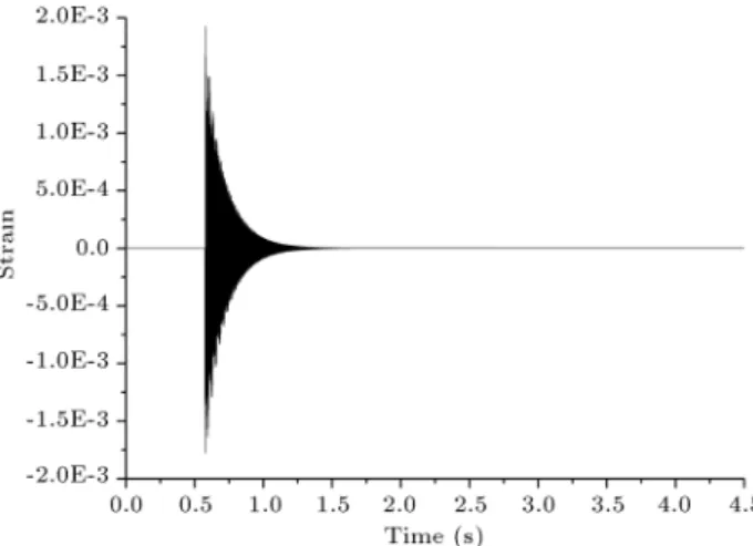
In this section, Scenarios 1 and 2 are used to choose the best excitation mode for the proposed damage identication. All damages are set to be DB = 0:25, and the stiness loss is set to be 3.52%. For hammer excitation, the hammer hits the beam at a speed of 4 m/s at time 0.575 s, and the recording lasts for 4.5 seconds. Figure 6 shows the strain-time history data of the midpoint. Figure 7 shows the instantaneous strain data of the entire beam at 0.01 s after the excitation by the hammer.
For running car excitation, the recording starts when the car starts to move from the left support and ends at 3.925 seconds after the car leaves the right support. The recording lasts for 4.5 seconds, the same as the hammer excitation. Figure 8 shows the strain-time history of the midpoint of the beam. Figure 9 shows the instantaneous strain of the xed end beam at 0.01 s after the car runs o the main beam.
Figure 10(a) shows the comparison between ham-mer excitation and running car excitation. Results show that the running car result is much better than the hammer excitation, especially at the supports.
Figure 6. Strain-time history data of hammer excitation.
Figure 7. Instantaneous strain at time 0.585 s of hammer excitation.
Figure 8. Time history data of running car excitation.
While the damage index of the hammer excitation reaches 0.05 at the supports, that of the running car excitation is almost zero, which means that the MWPER of a running car excitation is more stable than that of a hammer excitation.
The above-mentioned phenomenon is caused by the number of excitation points. The proposed method
Figure 9. Instantaneous strain at time 0.585 s of running car excitation.
Figure 10. Comparison between hammer excitation and running car excitation.
is capable of combining all the strain-time history data into one index for damage identication, meaning that the more points with larger strain exist, the more stable result we can obtain. With a running car excitation, every part could be excited, resulting in a large number of points with large strain, meaning better damage identication. Thus, for damage identications in a steel bridge, it is best that cars run from the left end
to the right end, i.e., the entire span of the beam, in order to collect enough response data.
5.1.3. Eects of dierent sensor intervals
In this section, Scenario 2 is used to examine the eect of sensor interval on the proposed damage identica-tion. All damages are set to be DB = 0:25, and the stiness loss is set to be 3.52%. There are three sensor intervals, i.e., 12.5 mm, 50 mm, and 200 mm, meaning that each sensor covers 12.5 mm, 50 mm, and 200 mm lengths of the beam, respectively.
As Figure 10(b) shows, the proposed damage index is capable of identifying damage with ve sensors on the beam, where the sensor interval is 200 mm. The identied damage locations are dierent. With 200 mm sensor intervals, the identied damage location is about 300 mm from the left support; with 50 mm sensor intervals, the identied damage location is about 225 mm from the left support; with 12.5 mm sensor intervals, the identied damage location is about 250 mm from the left support. While the actual damage location is DB = 250, the damage location identication errors can be explained and are acceptable. This phenomenon is caused by the sensors' mechanism. For long-gage ber optical sensors, the strain obtained is the average strain of the whole measure length, which means that as long as the damage location covered by sensors is applied, the strain change can be captured by the corresponding sensor. Since the x coordinate for each data point in Figure 10(b) is set to be the mid-point of corresponding sensor coverage length, the peak in Figure 10(b) means that there is a damage or damages in the corresponding sensor interval. Under the context that only 5 sensors or 20 sensors set up on the beam, Figure 10(b) shows that the proposed method is capable of identifying damages with only a few sensors.
5.1.4. Detectability of damages nearby the supports of the simply supported beam
In this section, Damage Scenario 3 is used to test if the second damage identication method is able to detect damages near the supports of a simply supported beam. The second damage identication method is based on strain signals. Since the strain values at the points near the supports of a simply supported beam are much lower than those at the points in the middle of the span, it becomes the main concern if damages that occur at points where the strain signals are weak can be identied.
Stiness loss of 3.52%, the same as those in the previous sections, is introduced on the simply supported beam. The car is run from the left side to the right side at a speed of 2 m/s. One damage is set to the left end of the simply supported beam. Another damage is set at a distance of 0.025 m from
Figure 11. The normalized MWPER of beams: (a) Damage at DB = 0 m and DB = 0:025 m, (b) the main beam with two damages, and (c) left front column.
the left support. Figure 11(a) shows that the damage at DB = 0:025 m can be identied, while the damage at DB = 0 m cannot be identied.
All the MWPERs are normalized in order to best estimate the damage location. Thus, the absolute values shown in Figure 11(a) are not of concern to us; only the relative values need to be of concern. The reason behind the fact that the strain in the elements near the supports of a simply supported beam is not totally zero, while strain of the elements at the support is almost zero, implies that all data in Figure 11(a)
are normalized. With FBG/BOTDR strain sensors, the results that are obtained represent the information gathered from the entire area covered by the sensors. Therefore, the strain change, caused by the damage, at DB = 0:025 m is detectible, while that of the damage at DB = 0 m is covered by other parts, whose strain value is much larger.
Since damages close to the hinge support can be identied, it can be concluded that as long as the damaged area is covered by a long-gauge strain sensor, and the strains on that area are not all zero, damages located at small strain areas can be identied. However, the damage will not be detected if the strain is too small, such as the strain on the elements located at the supports of a simply supported beam.
5.1.5. Detectability of multiple damages to the main beam and the damage to the column
In the next step, we explore if the concept behind the second method can be validated by applying this approach to multiple damage situations. In this section, this proposed concept is validated by the single layer frame model with two damages to the main beam. Since the running car excitation can only be applied to the main beam of the single layer frame, meaning that the columns cannot be excited directly, we will explore how damages to the columns can be taken into account and detected. Damage Scenario 4 is used to test if the proposed method can be used for this case or not.
Figure 11(b) and (c) show that all three damages are identied. Figure 11(b) indicates that multiple conditions are applicable for MWPER, which is pre-dictable since the strain is sensitive to local damage. Figure 11(c) shows that damages to a component that is not directly excited, i.e., the left column, are also detectable for MWPER. Thus, MWPER is an eective detection tool for application in steel bridges since all damages to all components can be identied.
5.1.6. Verication of the noise eect on the proposed method
All the results presented in this section are based on strain-time history data obtained from the nite element analysis of the response; hence, they contain no experimental noise. For real cases, experimental noise is inevitable. To evaluate the robustness of MWPER under measurement noise, the simulated data of Scenario 4 are contaminated with a certain level of articial random noise to generate `measured' data. Normally, distributed random noises, whose amplitudes are 5%, 10%, 30%, and 50% of the Root-Mean-Square (RMS) value of strain data, respectively, are added to the strain-time history data.
MWPERs in Figure 12(a) to (d) are normalized to make the comparison clear. With the increase of the
Figure 12. Normalized MWPER with dierent contaminated data: (a) Contaminated data (5%), (b) contaminated data (10%), (c) contaminated data (30%), and (d) contaminated data (50%).
noise level, disturbance on intact elements increases, especially on elements near the end points of the beam. It is important to note that even under a noise level of 30%, the damage can still be identied. This demonstrates that the second damage identication method is robust enough to take into account the measurement noise.
5.1.7. Eects of stiness loss level
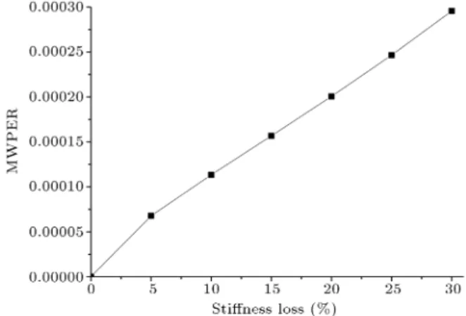
As stated in the previous sections, MWPER is capable of identifying the location of a damage under a certain noise level, which means the 2nd level of damage identication. In order to accomplish the 3rd level of damage identication and to show the ability of MWPER to quantify the damage, in this section, MWPERs of dierent stiness loss levels (3.52%, 5%, 10%, 15%, 20%, 25%, and 30%) are discussed.
Figure 13 shows the MWPERs on the 20th element changes with the change of stiness loss. As observed, the MWPERs also show a near-linear relationship with the stiness loss. Thus, with more stiness loss level of nite element data, MWPER is capable of identifying stiness loss level of a specic position. For a damage identication method to detect both the location and severity of a damage,
Figure 13. MWPERs of dierent stiness loss levels.
the relationship between the damage index and the location needs to be claried. As demonstrated in this case, the relationship between the location and the value of MWPER is estimated. Therefore, this approach is capable of detecting the severity of the damage, too.
5.1.8. Eects of damage location
Quantication of the damage needs a precise numerical relationship between the damage severity and the
dam-age index. In the previous section, it was veried that MWPER had a near-linear relationship with stiness loss. Therefore, the eects of the damage location need to be taken into consideration. In this section, Damage Scenario 2 is considered in order to explore and discuss the eects of damage location with the damage simulated by a stiness loss of 3.52%.
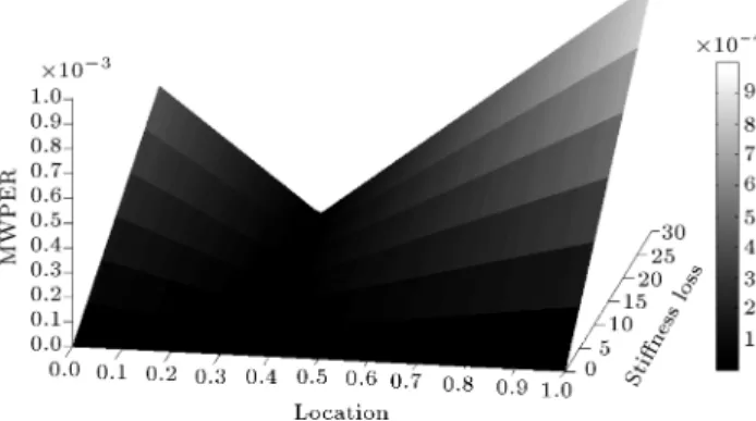
Since both the damage location and the damage level aect MWPER, the eects of damage location must be determined in order to make this damage identication method capable of determining damage level. Subsequently, the damage spanned across loca-tions DB = 0 to DB = 1 is simulated to determine the exact eects of the damage location on MWPER. Eighty damage locations were simulated to obtain the acquired results. Figure 14(a) shows the MWPER of damaged beams with damage locations spanning across DB = 0 to DB = 1.
5.1.9. Consideration of both damage location and damage level
In this section, both a simply supported beam and a xed end beam are used to calculate the relationship map among the location, damage severity, and location. Eighty damage location situations and 6 levels of stiness loss are considered, meaning that each beam's numerical model needs to be simulated for 80 6 = 480 times. In addition, there are two support conditions leading to 240 2 = 480 times of simulation. This requires an exhaustive computational time. Thus, to utilize ANSYS for this computation, a computation platform is set up, which consists of an Intel 4790K, 16GB DDR3 2200MHz, and a RAID0 disk array, in order to carry out a fast computation. Finally, these simulations form two damage index maps that can be used to identify damage severity.
As can be seen in Figure 14(b) and (c), the support conditions aect the distribution of MWPER. Thus, for dierent structures, dierent MWPER maps need to be established for the purpose of damage severity identication.
5.1.10. Consideration of modeling error
As discussed in the previous section, the identication of damage level needs a MPWER map generated by FEM simulation. The modeling-error must be taken into consideration, especially for its eect on the accuracy of damage severity identication. Based on Scenario 2, 6 modeling errors are tested. The stiness of the simulated beam changes to 80%, 90%, 110%, 120%, 130%, and 150% of the original stiness and, then, is tested. The result MWPERs are shown in Figure 15. The MWPER has a nearly linear relationship with the stiness change, almost the same as the index-damage relationship. The similar nearly linear relationships can be explained by the mechanism
Figure 14. MPWER of dierent damage scenarios: (a) Damage locations spanning across DB = 0 to DB = 1, (b) the simply supported beam, and (c) the xed ends beam.
Figure 15. MPWER of dierent damage scenarios on the xed ends beam.
of the proposed method. Both damage or modeling error will lead to the change of strain signal. In addition, their eects on strain amplitude are almost of the same degree, meaning that both the strain change caused by damage and that caused by modeling error will lead to the increase of MWPER.
Figure 15 and the discussion above show that modeling error has large impact on the accuracy of the proposed method. The modeling error must be limited with a small interval to ensure that the damage severity identication result is accurate.
5.1.11. Validation by a scaled single layer frame In this section, Scenario 4 is used to validate the proposed damage identication scheme. As stated in previous sections, by utilizing MWPER, location of all damages can be identied. Thus, the only information that needs to be obtained and validated is the capability of this approach in identifying the damage severity.
MWPER values of two damages to the main beam will be used as the reference to establish a damage index map. Subsequently, the index map will be utilized to identify the severity of the damage to the left front column.
Figure 16 shows the damage index map estab-lished for the left front column. As can be seen, its shape is between a simply supported beam and a xed ends beam. Based on the damage index map, the severity of the damage to the column can be identied. As noted earlier, the MPWER of the damage point on the column is 1.836E-4 and the damage location is at DLC = 0:5 m (Figure 15). Based on these two coordinates, the third coordinate in Figure 16 can be found, which is 22.36%. While the stiness loss in simulation is set to be 21.35%, the stiness loss value obtained via the MWPER map is 22.36%. Thus, the damage severity can be identied by MPWER. 6. Validation by experiment
The best way to determine if a damage identication method is good is always by applying it to a real
struc-Figure 16. Damage index map for left front column.
ture. Thus, in this work, an experiment is designed and run to determine whether the damage identication method works well or not. The experimental result showed that the proposed method was capable of identifying the damage in a real structure.
6.1. Design of the experiment
In order to validate the eectiveness of the proposed damage identication method, a simply supported steel beam is set up. The steel beam is an H-shape steel beam. The section of the bean is shown in Figure 17, where the length unit is chosen as mm. The length between two supports is 6000 mm (Figure 18(a)).
Usually, the xed ends supporting condition is dicult to reach, limited by the xation method. Besides, a simply supported support condition will lead to lower strain values nearby the supports, which is helpful for testing the eciency of the proposed method. Hence, a simply supported beam is set up as the main structure of this experiment.
As discussed earlier, commonly used long-gage strain sensors include FBG sensors and BOT-DER/BOTDA sensors. Both of them are capable of acquiring long-gage strain information from the structure. FBG sensors enjoy better accuracy in both dynamic and static sensing, while the sensing range limits FBG sensors. BOTDR/BOTDA sensors are suitable for long range sensing, such as a range of over several kilometers. However, the accuracy of BOTDR/BOTDA sensors is lower than FBG sensors. Considering that the steel beam is only 6 meters long, FBG sensors are used in this experiment.
The sampling rate is usually determined by the natural frequencies of the tested structure and sensing system properties. FBG sensors' sampling range can reach an extremely high value; thus, no limitation is placed on the decision of sampling rate. Then, the natural frequencies of the tested structure should
Figure 18. Design of the experiment: (a) The tested beam with sensors on both the top surface and bottom surface, and (b) damage introduced on top surface.
be considered as the only aspect that determines the sampling rate. According to numerical experiments, the rst three natural frequencies include 6.51 Hz, 10.65 Hz, and 31.94 Hz. Since the rst three natural frequencies are the most important for analysis, the sampling rate is set to be 1000 Hz, which is high enough to capture all vibration features of the beam.
This experiment aims to obtain sucient data. Hence, sensors, such as accelerometers, displacement meters, and FBG strain sensors, are installed on the tested beam. For the convenience of installation, FBG sensors are pasted on the bottom surface with displacement meters, while accelerometers are installed on the top surface of the tested beam. As can be seen in Figure 18(a), many sensors are distributed on the top and bottom surfaces of the tested beam. Thus, running car excitation is impossible for this tested beam. As a result, point excitation is adopted in this experiment. The excitation is introduced by a force hammer, which helps record the hammer force for the experiment.
In this experiment, the damage to the beam is in-troduced by cutting holes at top ange (Figure 18(b)). Since these holes cannot be cut accurately, the stiness
loss of the damage section is calculated after the cutting procedure. By accurate measurement and calculation, the stiness loss of the damaged section is determined to be 6.6%.
6.2. Experiment process
The FBG sensors used in this experiment have a sensing range of 1.5 m. Based on sensor parameters, number of sensors, and size of the tested beam, the tested beam is separated into 12 segments (E1, E2, ..., E12); each has a length of 0.5 m (Figure 19). The dividing points are used as excitation points; thus, there are 13 excitation points (H1, H2,...,H13). All these excitation points are shown in Figure 19. The damage is introduced to E3 by cutting holes on its top surface (Figure 18(b)).
The test procedure is run 24 times. As listed in
Table 2. Hammer force records. Test
number
Excited point
Without damage
With damage Hammer force (N) 1
H3
3622.82 2184.24
2 2615.97 2212.82
3 1907.02 2135.17
4
H5
2480.76 1537.82
5 2425.00 2093.90
6 2318.37 1883.47
7
H8
2402.75 1883.47
8 2056.68 2277.56
9 1768.33 1781.16
10
H9
1506.53 1871.52
11 1671.86 1677.18
12 1961.62 1744.82
Figure 20. Hammer force time history (Test 5).
Table 2, four excitation points are selected. Six tests are recorded for each excitation point, three for the intact status, and three for damaged status.
In order to match the damage index maps, all strain signals are normalized by setting the hammer force to 1. Table 2 shows the hammer force record of all these tests. Recorded data of Test 5 are shown in Figures 20 and 21. Figure 20 shows the hammer force time history of Test 5, which is quite clear. As can be seen in Figure 21, the strain signal is contaminated badly, with an error of about 10% of the largest strain. Figure 22 shows the instantaneous strain of both damaged and intact beams, and there is no signature that stands for the damage. Thus, the proposed damage identication method is utilized. 6.3. Damage identication based on the data
acquired by the experimental steel beam In this section, the data acquired during these exper-iments are applied to the proposed damage
identica-Figure 21. Strain time history of Test Number 5, intact: (a) Element 3, and (b) element 5.
Figure 22. Instantaneous strain at time of 10 s (Test 5).
tion scheme. Figure 22 indicates that the instantaneous strain distributions cannot show the damage location, while instantaneous strain distribution shows the dam-age location by slight disturbance on the curvature (Figures (7) and (9)). This phenomenon induces noise eects, as clearly shown in Figure 21.
A damage index map is presented for a simply supported beam (Figure 14(a)). However, the
excita-Figure 23. Damage index map for the tested beam.
Figure 24. Damage identication result of all 12 tests.
tion conditions are dierent; thus, a new damage index map is calculated and presented in Figure 23.
As can be seen, all experiments' data can be utilized to identify damage locations (Figure 24). The damage is shown clearly by peaks on element 3. How-ever, the MPWER value of each damage identication is dierent from another. This situation is hardened by noise eect since the noise cannot be denoised completely.
The next step of damage identication is to identify the damage severity. The damage is found on element 3, namely location 1.5 m. Although the MWPER values of dierent tests are dierent, they are considered to have the same importance to the damage identication result. Thus, the mean value of these 12 MWPER values is used for severity identication, which is 0.0407. Now, two coordinates of the damaged point on the damage index map are determined. Figure 25 shows the MWPER function in position 1.5 m. As can be seen in Figure 25, the stiness loss level is 10%, while the accurate damage level is 6.6%. Although there is a large dierence between the identied stiness loss and the accurate damage level, the noise eect in measured strain signals is relatively high; this result is acceptable.
Figure 25. MWPER function in position 1.5 m.
7. Concluding remarks
In this paper, MWPER was proposed for steel bridge damage identication based on long-gauge ber optic strain sensing. With both numerical and experimental validations, the proposed method proved to be suitable for the health monitoring of the entire structure. Moreover, the proposed method was robust to noise. As presented, the damage location could be identied under a noise level of up to 30%. Furthermore, it was clearly shown that the proposed scheme could be applied to identify multiple damage locations. It was also illustrated that the running car excitation was better than hammer excitation for the proposed damage identication method.
Based on the nearly linear relationship between MWPER and the stiness loss and the relationship between MWPER and the location, three damage index maps for damage identication were established for simply supported beam, xed end beam, and the left front column of the single layer frame. By utilizing these two maps, a corresponding map for single layer frame damage identication was established and tested. The test results showed that the proposed damage identication method was able to detect both location and severity of damages to steel bridges.
Acknowledgment
This research was supported by IIUSE of Southeast University by a grant provided by 1000 Program for the Recruitment of Global Experts. These supports are gratefully acknowledged.
References
1. Padgett, J.E. and Tapia, C. \Sustainability of nat-ural hazard risk mitigation: Life cycle analysis of environmental indicators for bridge infrastruc-ture", J. Infrastructure Systems, 19(4), pp.
395-408 (2013). https://doi.org/10.1061/(ASCE)IS.1943-5 55X.0000138.
2. He, C., Xing, J., Li, J., Qian, W., and Zhang, X. \A new structural damage identication method based on wavelet packet energy entropy of impulse response", The Open Civil Engineering Journal, 9, pp. 570-576 (2015).
3. Balageas, D., Fritzen, C.P., and Guemes, A., Structural Health Monitoring, Wiley-ISTE, London, pp. 493, ISBN: 978-1-905209-01-9 (2006).
4. Jiang, S.F., Wu, S.Y., and Dong, L.Q. \A time-domain structural damage detection method based on improved multiparticle swarm coevolution opti-mization algorithm", J. Mathematical Problems in Engineering, 2014, Article ID 232763, 11 pages, http://dx.doi.org/10.1155/2014/232763
5. Shi, Z.Y., Law, S.S., and Zhang, L.M. \Structural damage detection from modal strain energy change", J. Engineering Mechanics, 126(12), pp. 1216-1223 (2000).
https://doi.org/10.1061/(ASCE)0733-9399(2000)126: 12(1216).
6. Liu, Y., Fard, M.Y., and Chattopadhyay, A. \Dam-age assessment of CFRP composites using a time-frequency approach", J. Intelligent Material Systems and Structures, 23(4), pp. 397-413 (2012). DOI: https://doi.org/10.1177/1045389X11434171
7. Bu, J.Q., Law, S.S., and Zhu, X.Q. \Innovative bridge condition assessment from dynamic response of a passing vehicle", J. Engineering Mechanics - ASCE, 132(12), pp. 1372-1379 (2006).
https://doi.org/10.1061/(ASCE)0733-9399(2006)132: 12(1372).
8. McGetrick, P.J. and Kim, C.W. \Wavelet based dam-age detection approach for bridge structures utilis-ing vehicle vibration", In Proceedutilis-ings of 9th German Japanese Bridge, Symposium, GJBS09 (2012).
9. Gonzalez, A., Obrien, E.J., and McGetrick, P.J. \Iden-tication of damping in a bridge using a moving instru-mented vehicle", J. Sound and Vibration, 331(18), pp. 4115-4131 (2012).
https://doi.org/10.1016/j.jsv.2012.04.019.
10. Mallikarjuna Reddya, D., and Swarnamani, S. \Dam-age detection and identication in structures by spatial wavelet based approach", International Journal of Applied Science and Engineering, 10(1), pp. 69-87 (2012).
11. Wang, HF., Noori, M., and Zhao, Y. \A wavelet-based damage identication for large crane structures", Sixth World Conference on Structural Control and Monitoring, pp.15-17 (2014).
DOI: 10.13140/2.1.2810.7207
12. Hera, A. and Hou, Z. \Application of wavelet ap-proach for ASCE structural health monitoring bench-mark studies", J. Engineering Mechanics, 130(1), pp. 96-104 (2004). https://doi.org/10.1061/(ASCE)0733-9399(2004)130:1(96).
13. Gokdag, H. and Kopmaz, O. \A new damage detection approach for beam-type structures based on the combi-nation of continuous and discrete wavelet transforms", J. Sound and Vibration, 324(3), pp. 1158-1180 (2009). https://doi.org/10.1016/j.jsv.2009.02.030.
14. Hester, D. and Gonzalez, A. \A wavelet-based damage detection algorithm based on bridge acceleration re-sponse to a vehicle", J. Mechanical Systems and Signal Processing, 6(7), pp. 145-166 (2011).
https://doi.org/10.1016/j.ymssp.2011.06.007
15. Zhao, Y., Noori, M., Altabey, W.A., and Beheshti-Aval, S.B. \Mode shape based damage identication for a reinforced concrete beam using wavelet coecient dierences and multi-resolution analysis", J. Structural Control & Health Monitoring, 25(1), pp. 1-41 (2017). https://doi.org/10.1002/stc.2041
16. Zhao, Y., Noori, M., and Altabey, W.A. \Damage detection for a beam under transient excitation via three dierent lagorithms", J. Structural Engineering and Mechanics, 64(6), pp. 803-817 (2017).
DOI: https://doi.org/10.12989/sem.2017.64.6.803.
17. \Identication of hysterically degrading structures using the Bouc-Wen-Baber-Noori (BWBN) model", J.F. Silva Gomes and S.A. Meguid, Editors, Proceed-ings IRF2018: 6th International Conference Integrity-Reliability-Failure, Lisbon/Portugal, 22-26 July 2018, Publ. INEGI/FEUP, ISBN: 978-989-20-8313-1 (2018).
18. Reda Taha, M.M., Noureldin, A., Lucero, J.L., and Baca, T.J. \Wavelet transform for structural health monitoring: a compendium of uses and features", J. Structural Health Monitoring, 5(3), pp. 267-295 (2006). DOI: https://doi.org/10.1177/1475921706067741.
19. Nguyen, K.V. and Tran, H.T. \Multi-cracks detection of a beam-like structure based on the on-vehicle vi-bration signal and wavelet analysis", J. Sound and Vibration, 329(21), pp. 4455-4465 (2010).
https://doi.org/10.1016/j.jsv.2010.05.005.
20. Lee, S.G., Yun, G.J., and Shang, S. \Reference-free damage detection for truss bridge structures by con-tinuous relative wavelet entropy method", J. Struct. Health Monit, 145(2), pp. 28-45 (2014).
DOI: https://doi.org/10.1177/1475921714522845.
21. Li, S. and Wu, Z. \Characterization of long-gauge ber optic sensors for structural identication, smart structures and materials", International Society for Optics and Photonics, SPIE 5765, pp. 564-575 (2005). DOI: 10.1117/12.606367
22. Horiguchi, T., Kurashima, T., and Tateda, M. \Tensile strain dependence of Brillouin frequency shift in silica optical bers", Photonics Technology Letters, IEEE, 1(5), pp. 107-108 (1989).
DOI: 10.1109/68.34756.
23. Suzhen, L. and Zhishen, W. \Structural health mon-itoring strategy based on distributed ber optic sens-ing", J. Struct. Health Monit, 6(2), pp. 133-143 (2007). DOI: https://doi.org/10.1177/1475921706072078.
24. Dakin, J.P., Distributed Optical Fiber Sensor, Interna-tional Society for Optics and Photonics, SPIE 1797, pp. 76-108 (1993).
25. Lau, K.T., Yuan, L., and Zhou, L.M. \Strain mon-itoring in FRP laminates and concrete beams using FBG sensors", J. Composite Structures, 51(1), pp. 9-20 (9-2001).
https://doi.org/10.1016/S0263-8223(00)00094-5.
26. Schulz, W.L., Conte, J.P., and Udd, E. \Real-time damage assessment of civil structures using ber grat-ing sensors and modal analysis", 9th Annual Interna-tional Symposium on Smart Structures and Materials. International Society for Optics and Photonics, SPIE 4696, pp. 228-237 (2002).
27. Wei-Xin, R. and Sun, Z. \Structural damage iden-tication by using wavelet entropy", J. Engineering Structures, 30(10), pp. 2840-2849 (2008).
https://doi.org/10.1016/j.engstruct.2008.03.013.
28. Ovanesova, A.V. and Suarez, L.E. \Applications of wavelet transforms to damage detection in frame struc-tures", J. Engineering Structures, 26(1), pp. 39-49 (2004).
https://doi.org/10.1016/j.engstruct.2003.08.009.
29. Yongchao, Y. and Nagarajaiah, S. \Blind identication of damage in time-varying system using independent component analysis with wavelet transform", J. Me-chanical Systems and Signal Processing, 27, pp. 3-20 (2012).
https://doi.org/10.1016/j.ymssp.2012.08.029.
30. Jian-Gang, H., Ren, W., and Sun, Z. \Wavelet packet based damage identication of beam structures", In-ternational Journal of Solids and Structures, 42(26), pp. 6610-6627 (2005).
https://doi.org/10.1016/j.ijsolstr.2005.04.031.
31. Yen, G.G. and Lin, K.C. \Wavelet packet feature extraction for vibration monitoring", J. Industrial Electronics, IEEE Transactions on, 47(3), pp. 650-667 (2000).
DOI: 10.1109/41.847906.
32. Sun, Z., Chang, C.C. \Structural damage assessment based on wavelet packet transform", J. Structural Engineering, 128(10), pp. 1354-1361 (2002).
https://doi.org/10.1061/(ASCE)0733-9445(2002)128: 10(1354).
33. Han, J.G., Ren, W.X., and Sun, Z.S. \Wavelet packet based damage identication of beam structures", Int. J. Solids and Structures, 42(26), pp. 6610-6627 (2005). https://doi.org/10.1016/j.ijsolstr.2005.04.031.
34. Maosen, C. and Pizhong, Q. \Integrated wavelet transform and its application to vibration mode shapes for the damage detection of beam-type structures", J. Smart Materials and Structures, IOP, 17(5), pp. 222-232 (2008).
https://doi.org/10.1088/0964-1726/17/5/055014.
Biographies
Mohammad Noori is a Professor of Mechanical Engineering at California Polytechnic State Univer-sity, San Luis Obispo, California, USA. He is also a Distinguished Visiting National Chair Professor of 1000 Talent Program at the International Institute for Urban Systems Engineering, Southeast University, China. Prior to Cal Poly, Professor Noori served as a Higgins Professor and the Head of Mechanical Engineering at Worcester Polytechnic Institute, as an RJ Reynolds Professor and the Head of Mechanical and Aerospace Engineering at NC State University, and as a co-founder and Liasion Professor of National Institue of Aeroscape. He has served as the Chair of the ASME National Committee of Mechancial Engineering De-partment Heads, as a member of numerous US-Japan cooperative research programs, sponsored by NSF, and has received the Japan Society for the Promotion of Science Fellowship. He has served as a Program Direc-tor at NSF and has held leading positions in numerous national and international scientic organizations and professional societies. Noori has carried out original research work in nonlinear random vibrations and hys-teretic systems in multi-functional structures; for the past 15 years, his research has focused on the utilization of Ai-based schemes for structural health monitoring. He is an ASME Fellow, has published over 200 refereed papers, and serves as an executive editor, an associate editor, and an editorial board member of several jour-nals, as a technical advisor and board member of nu-merous scientic organizations and industries, and has delivered over 120 keynote and invited talks. He is an elected member of several professional honor societies. Haifegn Wang received Master's degree at Southeast University under the supervision of Professor Noori, a Distinguished Visiting National Chair Professor of China 1000 Talent Program at the International Insti-tute for Urban Systems Engineering, Southeast Univer-sity, China. He is currently a PhD student at the state University of New York in Bualo, USA.
Wael A. Altabey is an Assistant Professor of Me-chanical Engineering, Faculty of Engineering, Alexan-dria University, AlexanAlexan-dria, Egypt. He is currently an Associate Researcher and a visiting scholar at the International Institute for Urban Systems Engineering, in Southeast University and at Nanjing Zhixing In-formation Technology Co., Ltd., Nanjing, China. He was awarded a postdoctoral research certicate in 2018 after completing a post-doctoral research fellowship for two years, under the supervision of Professor Noori, in SHM and damage detection from Southeast University, Nanjing, China. Dr. Altabey received his PhD in 2015 in the area of fatigue of composite structures and his
MSc, 2009, in dynamic systems and his BSc, 2004, in Mechanical Engineering, from Mechanical Engineer-ing Department, Faculty of EngineerEngineer-ing, Alexandria University. Currently, Dr. Altabey is carrying out several projects related to the application of articial intelligence methods for structural health monitoring.
Ahmed I.H. Silik is currently a PhD student at the International Institute for Urban Systems Engineering, Southeast University, Nanjing, China. His research work involves the utilization of wavelet and articial neural network for the damage detection of reinforced concrete structures.